Index of Notations
| ${\Large\mathbb{N}}$ |
The set of natural numbers (or “counting numbers”), comprising $1$, $2$, $3$, $4$, etc: $$ \mathbb{N} = \{1, 2, 3, 4, \ldots\}. $$ Also known as the set of positive integers. Nb: positive means “greater than zero”; nonnegative means “zero or greater than zero”. |
|
| ${\Large \mathbb{Z}}$ |
The set of integers, comprising all natural numbers, their negatives, and zero: $$ \mathbb{Z} = \{\ldots, -3, -2, -1, 0, 1, 2, 3, 4, \ldots\}. $$ |
|
| ${\Large \mathbb{Q}}$ |
The set of rational numbers: all numbers that can be expressed as fractions of integers, such as $0.5 = \frac{1}{2}$, $4.137 = \frac{4137}{1000}$, $0.333333\ldots = 1/3$, $5 = 5/1$, $0 = 0/1$, and so on. A number is irrational if it is not in $\mathbb{Q}$. For example, $$ \sqrt{2\rule{0pt}{0.63em}} = 1.414213562373095... $$ happens to be irrational. (A not-so-obvious fact that requires a careful proof.) In general, a number is irrational if and only if its decimal expansion is infinite and non-repeating. |
|
| ${\Large \mathbb{R}}$ |
The set of
real numbers. This set includes any
number that |
|
| ${\Large \{\ldots\}}$ |
Curly brackets are used to list the elements of a set. For example, $$ A = \{1, 5\} $$ means that $A$ is a set containing (only) the numbers $1$ and $5$. |
|
| ${\Large \in}$ |
Means is an element of or (for short) is in. For example, $$ 1 \in \{1, 2\} $$ means “1 is in the set $\{1, 2\}$”; $$ 1.2 \in \mathbb{Q} $$ means “$1.2$ is in $\mathbb{Q}$” (or “$1.2$ is a rational number”); and $$ x \in \mathbb{R} $$ means “$x$ is in $\mathbb{R}$” (or “$x$ is a real number”). |
|
| ${\Large \notin}$ |
Means is not an element of, a.k.a., is not in. For example, $$ 3 \notin \{1, 2\} $$ since $3$ is not an element of the set $\{1, 2\}$, and $$ 0 \notin \mathbb{N} $$ since 0 is not a natural number, and $$ \sqrt{\hspace{0.02em}2\rule{0pt}{0.64em}} \notin \mathbb{Q} $$ since $\sqrt{2\rule{0pt}{0.63em}}$ is irrational. |
|
| ${\Large \subseteq}$ |
Means is a subset of. I.e., $$ A \subseteq B $$ means that every element of $A$ is an element of $B$. For example, $$ \mathbb{N} \subseteq \mathbb{N} $$ (every set is a subset of itself), or $$ \mathbb{N} \subseteq \mathbb{Z} \subseteq \mathbb{Q} \subseteq \mathbb{R} $$ because $\mathbb{N}$ is a subset of $\mathbb{Z}$, $\mathbb{Z}$ is a subset of $\mathbb{Q}$, and $\mathbb{Q}$ is a subset of $\mathbb{R}$. The difference between $$ \rm{“}A \in \mathbb{R}\rm{”} \qquad \rm{and} \qquad \rm{“} A \subseteq \mathbb{R} \rm{”} $$ is the difference between “$A$ is in $\mathbb{R}$” (i.e., $A$ is a real number) and “$A$ is a subset of $\mathbb{R}$” (i.e., $A$ is a set of real numbers). |
|
| ${\Large \Rule{0.71pt}{0.5em}{0.02em}\hspace{0.08em}x\hspace{0.08em}\Rule{0.71pt}{0.5em}{0.02em}}$ |
The absolute value of $x$. E.g., $|\!-\!5| = 5$, $|5| = 5$, $|0| = 0$, $|\!-\!10.3| = 10.3$. (Strips away minus signs.) |
|
| ${\Large \phi}$ |
The empty set. A set with no elements. |
|
| ${\Large \{\}}$ |
A different notation for the empty set. (I.e., $\phi = \{\}$.) |
|
| ${\Large \infty}$ |
Infinity. (Informal; not a number.) |
|
| ${\Large :}$ |
Such that. For example, $$ \{x \in \mathbb{R} : 0 \leq x \leq 3\} $$ is “the set of all $x \in \mathbb{R}$ such that $0 \leq x \leq 3$”, i.e., “the set of all real numbers $x$ such that $0 \leq x \leq 3$”. Similarly, $$ \{q \in \mathbb{Q} : q^2 < 2\} $$ is “the set of all rational numbers $q$ such that $q^2 < 2$”. |
|
| ${\Large [a,b]}$ |
The closed interval delimited by $a$ and $b$: $$ [a,b] = \{x \in \mathbb{R} : a \leq x \leq b\}. $$ For example, $$ [0,1] $$ is the set of all real numbers that are greater than or equal to 0 and less than or equal to 1. |
|
| ${\Large (a,b)}$ |
The open interval delimited by $a$ and $b$: $$ (a,b) = \{x \in \mathbb{R} : a < x < b\}. $$ Can also be used with $a = -\infty$, $b = \infty$, or both: $$ \begin{align} (-\infty, b) &= \{x \in \mathbb{R} : x < b\},\\ (a, \infty) &= \{x \in \mathbb{R} : a < x\},\\ (-\infty, \infty) &= \mathbb{R}. \end{align} $$ |
|
| ${\Large [a,b)}$ |
The half-open interval that is closed at $a$ and open at $b$: $$ [a,b) = \{x \in \mathbb{R} : a \leq x < b\}. $$ Can also be used with $b = \infty$: $$ [a, \infty) = \{x \in \mathbb{R} : a \leq x\}. $$ |
|
| ${\Large (a,b]}$ |
The half-open interval that is open at $a$ and closed at $b$: $$ (a,b] = \{x \in \mathbb{R} : a < x \leq b\}. $$ Can also be used with $a = -\infty$: $$ (-\infty, b] = \{x \in \mathbb{R} : x \leq b\}. $$ |
|
| ${\Large \iff}$ |
If and only if. For example, $$ (x \in \mathbb{N}) \iff (x \in \mathbb{Z}, x > 0) %(x \in \mathbb{W}) \iff (x \in \mathbb{Z}, x \geq 0) $$ reads “$x$ is a natural number if and only if $x$ is an integer, greater than or equal to zero”. |
|
| ${\Large \Longrightarrow}$ |
Implies. For example, $$ (x \in \mathbb{Z}) \Longrightarrow (x \in \mathbb{Q}) $$ can be read “the fact that $x$ is an integer implies that $x$ is a rational number”, or $$ (x \in (0,1]\hspace{0.04em}) \Longrightarrow (x \ne 0) $$ can be read “the fact that $x$ is in the half-open interval $(0,1]$ implies that $x$ is nonzero”. |
|
| ${\LARGE \cup}$ |
Union. E.g., $$ \{1, 2\} \cup \{2, 3\} = \{1, 2, 3\} $$ and $$ \mathbb{Z} \cup \mathbb{N} = \mathbb{Z} $$ because $\mathbb{N}$ adds nothing new to $\mathbb{Z}$ (i.e., $\mathbb{N} \subseteq \mathbb{Z}$). |
|
| ${\LARGE \cap}$ |
Intersection. E.g., $ \{1, 2\} \cap \{2, 3\} = \{2\} $, $ (-1,1] \,\,\cap$ $[0,2) = [0,1]. $ |
|
| ${\Large \backslash}$ |
Remove. For example, $$ \{1, 2\} \backslash \{2, 3 \} = \{1\} $$ as 1 is the only element of $\{1, 2\}$ that is not in the set $\{2, 3\}$, or, $$ \mathbb{R}\backslash\{0\} = (-\infty, 0) \cup (0, \infty) $$ as removing the number 0 from $\mathbb{R}$ leaves us with the union of the two open intervals $(-\infty,0)$ and $(0,\infty)$. |
Bootcamp 2: Powers of 10
Terminology. The expression below is called a power; the number at the bottom of the power is called the base (of the power); the number at the top is called the exponent:

The whole expression is read $\mathit{10}$ to the power $\mathit{3}$, and the general process of taking a power is called exponentiation.
Integer powers of 10. We define $$ \Large 10^{\hspace{0.2ex}n} $$ as follows, if $n$ is a nonnegative integer: start from $1$ and multiply by $10$ $n$ times. We also define $$ \Large 10^{-n} $$ as follows, if $n$ is a positive integer: start from $1$ and divide by $10$ $n$ times.
For example, $$ \Large 10^4 = 1 \times 10 \times 10 \times 10 \times 10 = 10000 $$ $$ \Large 10^3 = 1 \times 10 \times 10 \times 10 = 1000 $$ $$ \Large 10^2 = 1 \times 10 \times 10 = 100 $$ $$ \Large 10^1 = 1 \times 10 = 10 $$ $$ \Large 10^0 = 1 = 1 $$

(where, in the last line, $1$ is multiplied by $10$ zero times, as per the exponent, which is zero) by the first definition, while $$ \Large 10^{-1} = 1\,/\,10 = 0.1 $$ $$ \Large 10^{-2} = (1\,/\, 10)\,/\,10 = 0.01 $$ $$ \Large 10^{-3} = ((1\,/\, 10)\,/\,10)\,/\,10 = 0.001 $$ $$ \Large 10^{-4} = (((1\,/\, 10)\,/\,10)\,/\, 10)\,/\, 10 = 0.0001 $$ by the second definition.
As $n$ successive divisions by $10$ is the same as one division by $10^n$, one also has $$ \Large 10^{-n} = {1 \over 10^{\hspace{0.2ex}n}}\tag{*} $$ for every positive integer $n$, which gives an alternate means of computing $10^{-n}$. Moreover, (*) actually holds for
every

integer $n$, which is mildly important. In more detail, (*) holds for $n = 0$ by inspection, and (*) is equivalent to the identity $$ \Large 10^{-n}10^n = 1 \tag{**} $$
which holds for $n$ if and only if it holds for $-n$. (By which we mean: replacing “$n$” by “$-n$” in (**) lands you right back on (**), due to the fact that $-{(-n)} = n$.) (So, namely, if (**) holds for all positive values of $\hspace{0.05em}n$, then it holds for all negative values of $n$, as well.)
Vocabulary. Numbers $a$ and $b$ such that $$ \Large ab = 1 $$ are reciprocal. If $a$ and $b$ are reciprocal, then these equations are satisfied... $$ \Large ab = 1 \qquad a = {1 \over b} \qquad b = {1 \over a} $$ ...and any one of these equations implies the other two. Thus, either of (*) and (**) expresses the
reciprocality
of $10^n$ and $10^{-n}$.
Other bases. Integer powers of other nonzero bases are defined similarly, e.g., $$ \Large 2^{-2} $$ is defined as $1$ divided by $2$ twice, etc.
However, a small quirk occurs for base $0$: as one cannot divide by $0$, negative powers of $0$ remain undefined. E.g., $$ \Large 0^{-2} $$ would be “$1$ divided by $0$ twice”, but this is undefined. Hence $0^{-1}$, $0^{-2}$, etc, remain undefined.
Also (in case you're wondering) $0^0 = 1$. You can see this by writing down the first few powers of $0$ in descending order: $$ \Large 0^3 = 1 \times 0 \times 0 \times 0 = 0 $$ $$ \Large 0^2 = 1 \times 0 \times 0 = 0 $$ $$ \Large 0^1 = 1 \times 0 = 0 $$ $$ \Large 0^0 = 1 = 1 $$ In other words, every positive power of $0$ is zero, but when it comes to $0^0$, the ‘$0\hspace{0.12ex}$’ in the exponent “wins out” over the ‘$0\hspace{0.12ex}$’ in the base, making the result $1$.
Note that mathematicians sometimes refer to a power with an exponent of $0$ as an
empty product
and they will repeatedly admonish that
an empty product is $\mathit{1}$
in the sense that “all products start at $1$”, and that if you start at $1$ and don't multiply anything in, you stay at $1$.
Additivity of exponents. If you think about it, $$ \Large 10^{13} \times 10^{14} = 10^{\hspace{0.1ex}27} $$ because $13$ multiplications by $10$ followed by $14$ multiplications by $10$ makes $13 + 14 = 27$ multiplications by $10$.
More generally, $$ \Large 10^{\hspace{0.1ex}n} \times 10^{\hspace{0.1ex}m} = 10^{\hspace{0.1ex}n + m} $$ for all $n$ and $m$ (and other bases than $10$), which is known as
additivity of exponents
and which is sometimes paraphrased by saying that
the product of the powers is the power of the sum
where the product of the powers refers to “$10^n \times 10^m$” and the power of the sum refers to “$10^{n+m}$”. (Or for some other base.)
The third law of exponents. Also, if you think about it, $$ \Large (10^{13})^{14} = 10^{13\cdot 14} $$
because multiplying $14$ times by $10^{13}$ is like multiplying $13\cdot 14$ times by $10$. More generally, $$ \Large (10^n)^m = 10^{nm} $$ for all $n$ and $m$. This is known as “the third law of exponents”.
On this subject, note that if one writes $$ \Large a^{b^{c}} $$ [“$a$ to the power $b$ to the power $c$”] there is a seeming ambiguity: does it mean $$ \Large a^{\left(b^{c}\right)} $$ [“$a$ to the power [$b$ to the power $c$]”] or does it mean $$ \Large (a^{b})^{c} $$ [“[$a$ to the power $b$] to the power $c$”]...? Well, because the second way can be written $$ \Large a^{bc} $$ by the third law of exponents, the second way already has “its own” notation, and therefore the convention is that... $$ \Large a^{b^c} $$ ...absolutely always means... $$ \Large a^{\left(b^c\right)} $$
...!
Famous powers of 10. Many human languages have special names for various integer powers of $10$, due to the fact that many of our ancestors chose to count in base $10$.
In English, e.g., these are some of the “famous” powers of $10$:
| $n$ | $\,\,10^n$ | name |
| $0$ | $1$ | one |
| $1$ | $10$ | ten |
| $2$ | $100$ | hundred |
| $3$ | $1000$ | thousand |
| $6$ | $1\,000\,000$ | million |
| $9$ | $1\,000\,000\,000$ | billion |
| $12$ | $1\,000\,000\,000\,000$ | trillion |
One can note that
one million is a thousand thousand
because $$ \Large 1000 \times 1000 = 1000\hspace{0.3ex}000 $$ by counting zeroes, or, equivalently, because $$ \Large 10^3 \times 10^3 = 10^6 $$ by additivity of exponents. Similarly, note that
one billion is a thousand million

and
one trillion is a thousand billion

and also (while we're at it)
one trillion is a million million

as can be seen, for example, by replacing “billion” with “thousand million” in the previous sentence and then further replacing “thousand thousand” with “million” in that sentence.
Negative exponent prefixes. For negative exponents we simply say “one tenth” instead of “ten”, etc. Specifically, the table looks like so:
| $n$ | $\,\,10^n$ | name |
| $-1$ | $0.1$ | one tenth |
| $-2$ | $0.01$ | one hundredth |
| $-3$ | $0.001$ | one thousandth |
| $-6$ | $0.000\,001$ | one millionth |
| $-9$ | $0.000\,000\,001$ | one billionth |
| $-12$ | $0.000\,000\,000\,001$ | one trillionth |
In passing, note how the standard decimal expansion for $10^{-1}$ contains exactly one ${0}$:

Likewise, the standard decimal expansion for $10^{-2}$ contains exactly two $0$'s...

...and so on, which is a possible trick to check one's work and avoid mistakes.
However, there also exist negative exponent
prefixes
that people use to qualify other measures. For example, a
millimeter
is $10^{-3}$ meters, i.e., one thousandth of a meter, because “milli” happens to be the prefix for $10^{-3}$. Here is a list of the most common such prefixes:
| power | prefix |
| $10^{-1}$ | deci |
| $10^{-2}$ | centi |
| $10^{-3}$ | milli |
| $10^{-6}$ | micro |
| $10^{-9}$ | nano |
| $10^{-12}$ | pico |
| $10^{-15}$ | femto |
(Funny how the prefixes switch from ending in ‘i’ to ending in ‘o’ after $10^{-3}$.) (Well, anyway.)
To give an idea of scale,
micrometers
are smaller than the smallest animal cells (human red blood cells, which are among the smallest animal cells, have a diameter of $7$~$9$ $\mu\textrm{m}$) (nb: “$\mu$” stands for “micro” and “$\mu$m” stands for “micrometer”). Next down,
nanometers
happen to be smaller than the diameter of DNA, with DNA having a diameter of about $2.5$nm (“nm” = “nanometer”).
Positive exponent prefixes. There exists a similar set of prefixes for positve powers of $10$. Going up to $10^{15}$, these are:
| power | prefix |
| $10^{1}$ | deca |
| $10^{2}$ | hecto |
| $10^{3}$ | kilo |
| $10^{6}$ | mega |
| $10^{9}$ | giga |
| $10^{12}$ | tera |
| $10^{15}$ | peta |
For example, a
kilometer
is a thousand meters [b/$\!\hspace{0.1ex}\rm{c}$ “kilo” = thousand], while a
terabyte
is a trillion bytes [b/$\!\hspace{0.1ex}\rm{c}$ “tera” = trillion]. (In case you don't know, by the way, a
byte
is a unit of computer memory that is equal to $8$ bits, with a bit being a single 0/1 value.)
Logarithms base 10. Every positive number can be uniquely written as “ten to the power something”. This “something” will heretofore be called the logarithm base $\mathit{10}$ of that (positive) number.
For example, $$ \Large 100 $$ can be uniquely written as “ten to the power something”. To wit, $100$ is, of course,
ten to the power $\mathit{2}$
and this means that $$ \Large 2 $$ is the logarithm base $10$ of $100$.
Example 1. It so happens that $$ \Large 99 = 10^{1.99563519...} $$ under an extended definition of exponentiation that allows us to compute $10^x$ for every $x \in \mathbb{R}$. So $$ \Large 1.99563519... $$ is the logarithm base $10$ of $99$.
Example 2. It so happens that $$ \Large 98 = 10^{1.99122607...} $$ under the same extended definition, so $$ \Large 1.99122607... $$ is the logarithm base $10$ of $98$.
Example 3. Since $$ \Large 0.1 = 10^{-1} $$ the logarithm base $10$ of $0.1$ is $-1$.
Example 4. Since $$ \Large 0.00001 = 10^{-5} $$

the logarithm base $10$ of $0.00001$ is $-5$.
Bootcamp 1: Sets
Notation. Curly braces typically denote the beginning “$\{$” and ending “$\}$” of a collection of elements, otherwise known as a set. For example, this is a set containing the numbers $1$, $2$ and $3$ (and nothing else): $$ {\Large\{1, 2, 3\}} $$ Also, $$ {\Large\{1\}} $$ is a set containing just the number $1$, while $$ {\Large\{1, 3\}} $$ is a set containing just the numbers $1$ and $3$, etc. Even, $$ {\Large\{\}} $$ is an empty set, a set with no elements!
What it does. The “API” (a computer science notion, roughly meaning
the interface offered to the outside world
as in, for example, the buttons and clock display and door handle of a microwave oven) of a set consists of just one functionality: a set can answer questions of the form
do you contain ... ?
and nothing else. For example, you could ask a set
do you contain 3?
to which $\{1, 3\}$ would answer “yes”, but $\{ 1\}$ would answer “no”, or
do you contain 2?
to which $\{1\}$ and $\{1, 3\}$ would both answer “no”, but $\{1, 2, 3\}$ would answer “yes”.
Notation-wise, the expression $$ {\Large x \in A} $$ means
$A$ contains $x$
or
$A$ answers “yes” to the question “do you contain $x$?”
equivalently. [One can also say
$x$ in $A$
or
$x$ is in $A$
or
$x$ is an element of $A$
depending on one's mood and/or tastes.] As in all of mathematics, any such statement evaluates to either “true” or “false”. For example, $$ {\Large 1 \in \{1, 2\}} $$ is true, because $1$ is an element of the set $\{1, 2\}$, whereas $$ {\Large 3 \in \{1, 2\}} $$ is false, because $3$ is not an element of the set $\{1, 2\}$.
Set Equality. Two sets are deemed to be equal if and only if they answer the same to all “do you contain ...?” questions. For example, while $$ {\Large\{2, 1\}} $$ might look superficially different from $$ {\Large\{1, 2\}} $$ these sets are actually one and the same, because they both answer “yes” to
do you contain 1?
do you contain 2?
and answer “no” to all else. For that matter, $$ {\Large\{1, 1, 2\}} $$ might also look superficially different from $$ {\Large\{1, 2\}} $$ but since both sets answer “yes” to
do you contain 1?
do you contain 2?
and answer “no” to all else, they are by definition the same.
(These examples demonstrate that human notation is redundant: there are several different ways of writing down the same set. They also demonstrate that sets do not keep track of the
order
nor of the
multiplicity
of their elements. Such notions are simply not part of the “API” of a set.)
Moreover, any empty set is equal to any other empty set. Equality follows because both sets answer all questions the same way: they both answer “no” to everything. So there is
one
and only one empty set. Therefore, mathematicians speak of
the
empty set—the one and only!
Second notation for the empty set. While the empty set can be written $$ {\Large \{\}} $$ another available notation is $$ {\Large \phi} $$ which is the Greek letter phi, read “fee”. (Or “fie”? Hum.) (Or you can just say “the empty set”, and keep it safe.)
Sets within sets. Sets can be nested much like Russian dolls. In fact, the result of doing this might even look like a little bit like a Russian doll (no?): $$ {\Large \{\{\{\{\}\}\}\}} $$ The above is “a set containing a set containing a set containing a set containing the empty set”. Eschewing complete adherence to the Russian doll aesthetic, we could also write $$ {\Large \{\{\{\phi\}\}\}} $$ for the same thing, given that $\phi = \{\}$.
Mind you, concerning this example, that $$ {\Large \{\{\} \} \ne \{\}} $$

because a box containing an empty box is not the same thing as an empty box! Specifically, $$ {\Large \{ \{\} \}} $$ answers “yes” to the question “do you contain $\{\}$?” (a.k.a., “do you contain $\phi$?”) whereas $$ {\Large \{\}} $$ answers “no” to the same question. (Indeed, while the empty set contains nothing, it is something.) Similarly, $$ {\Large \{\{\{\}\} \} \ne \{\{\}\}} $$ etc, etc: adding a new outer layer changes the whole set each time.
Set union and set intersection. The so-called union of two sets $A$ and $B$ is written $${\Large A \cup B}$$ and consists of the set of all things that are either in $A$ or in $B.$ For example, $$ {\Large \{1, 2\} \cup \{2, 5\} = \{1, 2, 5\}} $$ as $1$, $2$ and $5$ are the only elements to find themselves either in $\{1, 2\}$ or in $\{2, 5\}$. The so-called intersection of two sets $A$ and $B$ is written $${\Large A \cap B}$$ and consists of the set of all things that are both in $A$ and in $B$. For example, $$ {\Large \{1, 2\} \cap \{2, 5\} = \{2\}} $$
as $2$ is the only element that is both in $\{1, 2\}$ and in $\{2, 5\}$.
Note that $$ {\Large x \in (A \cup B)} $$ if and only if $$ {\Large x \in A} $$ or $$ {\Large x \in B} $$ because that's how we defined “union”. (Replace “or” by “and” to get a definition of intersection.) In fact, a logician would define the union of two sets by an abstruse expression of the type $$ {\Large x \in (A \cup B) \iff (x \in A) \vee (x \in B)} $$ read
an element $x$ is in the thing I call “$A \cup B$”
if and only if $x$ is in $A$ or $x$ is in $B$
as “$\!\!\iff\!\!$” means “if and only if” and “$\vee$” means “or”. (You can figure out the similar definition for the intersection of two sets if we tell you that $$ {\Large \wedge} $$ means “and”.)
Sets encountered in calculus. In calculus, you will see sets such as the real numbers $$ {\Large\mathbb{R}} $$ which is an infinite set containing all “ordinary” decimal numbers, or such as the integers $$ {\Large\mathbb{Z}} $$ which contains all “whole” numbers, including the negative ones. You might also encounter the natural numbers $$ {\Large\mathbb{N}} $$ which contains only those integers that are greater than $0$ (i.e., $\mathbb{N}=\{1, 2, 3, \ldots \}$).
Secondly—and this pretty much wraps it up for those sets that are commonly seen in calculus—you will encounter intervals. For example, $$ {\Large [a, b]} $$ is a closed interval, consisting of all (real) numbers greater than or equal to $a$, and less than or equal to $b$. Or $$ {\Large [a, b)} $$ is a half-open interval, consisting of all real numbers greater than or equal to $a$, and less than $b$. Etc.
Note that $$ {\Large (-\infty, \infty) = \mathbb{R}} $$ since $$ {\Large (-\infty, \infty)} $$ (which is an open interval, by the way) means
the set of real numbers with no bound below,
and no bound above
which is all of $\mathbb{R}$.
Sets not encountered in calculus. If you take a more advanced course, you might encounter the so-called set of extended real numbers, written $$ {\Large\overline{\mathbb{R}}} $$ and which consists of all the numbers in $\mathbb{R}$, plus the formal symbols “$-\infty$”, “$\infty$” as well: $$ {\Large\overline{\mathbb{R}} = \mathbb{R} \cup \{-\infty, \infty\}} $$ (I.e., ...well, you get it!)
You can view $\overline{\mathbb{R}}$ as a kind “closed interval” version of $\mathbb{R}$, that is, think of $\overline{\mathbb{R}}$ as being the closed interval $$ {\Large [-\infty, \infty]} $$ with the two infinite endpoints included.
Does all this have any “real meaning”? Good question! The answer is: not until you give it one.
E.g. (to give you a brief flavor, before we move on forever from the topic), the value of something like $$ {\Large 0.5+ \infty} $$ must be defined. (It is defined to be $\infty$, in case you're curious. In fact, one has $a + \infty = \infty$ for any $a \ne -\infty$.) And some things remain explicitly undefined. For example, the expression $$ {\Large (-\infty) + \infty} $$ has an undefined value—the same way, say, that division by $0$ is undefined in $\mathbb{R}$.
Chapters
Chapter 1: A Few Refreshers
Chapter 2: Slopes
Chapter 3: Functions
Chapter 4: Derivatives
Chapter 5: Cos and Sin
Bootcamps
Bootcamp 1: Sets
Bootcamp 2: Powers of 10
Index of Notations
Chapter 1: A Few Refreshers
Square Roots. You might remember that “minus times minus is plus” and that “plus times plus is plus”. (Why? The enemy of my enemy is my friend.) So any nonzero number multiplied by itself is positive. For example, $$ (-2) \times (-2) = 4 $$
$$ 2 \times 2 = 4 $$ are both positive. But $\sqrt{4}$ is, by definition, the unique nonnegative solution to $x^2 = 4$. Hence, and whether you like it or not,
 $$
(-2)^2 = 4,\,\, \sqrt{4} = 2
$$
$$
(-2)^2 = 4,\,\, \sqrt{4} = 2
$$
and, in particular, it is not true that $$ \sqrt{x^{2}} \,=\, x $$ for every real number $x$. Instead we have $$ \sqrt{x^{2}} \,=\, |x| $$ for every real number $x$, where $|x|$ denotes the absolute value of $x$.
(Nb: If ever you want to indicate both solutions of the equation $x^2 = 4$ you can always use the notation “$\pm \sqrt{4}$”. This is what happens, for example, in the maybe-well-known formula $$ x = {-b \pm \sqrt{b^2 - 4ac} \over 2a} $$
for the solutions to the quadratic equation $ax^2 + bx + c = 0$.)
Now we can ponder, say, $$ \sqrt{0.5} $$ whose value is—by definition—the unique nonnegative solution to $$ x^2 = 0.5. $$ As beginners, there's nothing wrong with trying to solve this equation by trial and error. With $x = \frac{1}{4}$, for example, we find $$ x^2 = \frac{1}{4}\times\frac{1}{4} = \frac{1}{16} $$ so $x = \frac{1}{4}$ is not a solution of the equation, being apparently too small. Increasing $x$ to $x = \frac{1}{2}$, say, we find $$ x^2 = \frac{1}{2}\times\frac{1}{2} = \frac{1}{4} $$ which is better, since $1/4$ is closer to $1/2$, but still too small. Increasing $x$ by $1/4$ again, say, to $x = \frac{3}{4}$, we find $$ x^2 = \frac{3}{4}\times\frac{3}{4} = \frac{9}{16} $$ which—surprise!—is actually pretty close to $1/2$, as $1/2 = 8/16$. And since $9/16 > 0.5$, $\sqrt{0.5}$ must be a little less than $\frac{3}{4} = 0.75$.
In last resort, and in reasonably good agreement with our observations, a calculator reveals that $$ \sqrt{0.5} = 0.7071067... $$ where the decimals trail off with no pattern. (This number is irrational.) Even so, the fact that $\sqrt{0.5}$ is greater than $0.5$ is often perceived as counterintuitive.
You can think of it this way: multiplying a value by $0.7071$, or approximately $\sqrt{0.5}$, is like taking $70.71\%$ of that value—for example, say, $$ 605\cdot 0.7071 = 427.7955 $$ is $70.71\%$ of $605$, and so on—so if we multiply twice by $0.7071$ we obtain “$70.71\%$ of $70.71\%$” and it just so happens that “$70.71\%$ of $70.71\%$” is close to $50\%$.
The point is: if “$X\%$ of $X\%$” equals $50\%$, then, of course, $\hspace{0.03em}X > 50$—that much seems logical—and, with a little thought, the same phenomenon explains why $\sqrt{0.5} > 0.5$.
Fractions and Division. An elementary fraction, or division, such as $$ {50 \over 2} $$ can be thought of in a few different ways:
- Fifty halves (i.e., $50 \times \frac{1}{2}$).
- The size obtained when something of size fifty is divided into two equal parts (answer: $25$).
- The number of times that $2$ goes into $50$ (answer: $25$, because it takes twenty-five $2$'s to make up $50$).
But $50/2$ is a ratio of integers, which makes things particularly nice! For a ratio of decimals, such as, say, $$ {1 \over 0.01} $$ our possible points of view are going to be more restricted. Thankfully, however, we can still characterize this fraction as the answer to the question “how many times does $0.01$ go into $1$?” as in the third option above. And, indeed, $$ {1 \over 0.01} \,=\,100 $$ because $0.01$ goes $100$ times into $1$. For that matter, $$ { 1 \over 0.001} = 1000,\qquad{1 \over 0.0001} = 10000,\quad\,\,\,\,\textrm{(etc)} $$ by the same reasoning, which explains why dividing by smaller and smaller numbers produces larger and larger results (and, by extension, why dividing by $0$ is undefined).
Note. In general, the ratio of two decimal numbers can be turned into a ratio of integers by multiplying the ratio top and bottom by a suitable power of $10$. E.g.: $$ {1.42 \over 0.8} = {100 \cdot 1.42 \over 100 \cdot 0.8} = {142 \over 80} = {71 \over 40}. $$ This example was chosen randomly, and, if you allow, we would like to see how large $71/40$ really is (one second!): $$ \begin{align} {71 \over 40} \,&=\, {40 + 30 + 1 \over 40} \,=\, {40 \over 40} + {30 \over 40} + {1 \over 40}\\ \,&=\, 1 + {3 \over 4} + {1 \over 4}\!\cdot \!{1 \over 10}\rule{0pt}{1.5em}\\ \,&=\, 1 + 0.75 + 0.025 = 1.775\rule{0pt}{1.5em} \end{align} $$ ...so we find, among others, that $71$ is exactly $77.5\%$ greater than $40$. (Interesting, no?)
Distributivity. As you might already know, a number that multiplies a sum can be brought “inside” the sum. For example, $$ 5(10 + 2) \,=\, 5\!\cdot\!10 \,+\, 5\!\cdot\!2 $$ (five times twelve equals fifty plus ten), or $$ a(b + c) = ab + ac $$ more generally. This property is known as the distributivity of multiplication over addition, or distributivity for short.
(We might finally clarify that ‘$\cdot$’ means “times”, i.e., the same as ‘$\times$’. Moreover, when we write $$ 5\!\cdot\!10 \,+\, 5\!\cdot\!2 $$ we really mean $$ (5\!\cdot\!10) + (5\!\cdot\!2) $$ as opposed to something else, such as $$ ((5\!\cdot\!10) + 5)\!\cdot\! 2, $$
because multiplication takes precedence over addition, by default.)
A little more generally, one has such identities as $$ (a + b)(C + D) \,=\, aC + bC + aD + bD $$

that come from multiplying every term of the first parenthesis with every term of the second parenthesis. Indeed, $$ (a + b)(C + D) = (a + b)C + (a + b)D $$ by one application of distributivity, while $$ (a + b)C = aC + bC $$ $$ (a + b)D = aD + bD $$ by distributivity again.
Example 1. One has $$ \begin{align} (10 + 2)(10 + 4) \,&=\, 10\!\cdot\!10 \,+\, 10\!\cdot\!4 \,+\, 2\!\cdot\!10 \,+\, 2\!\cdot\!4\\ \,&=\, 100 \,+\, 40 \,+\, 20 \,+\, 8\\ \,&=\, 168 \end{align} $$ so $12 \times 14 = 168$.
Example 2. One has $$ \begin{align} (10 + 3)(10 + 3) \,&=\, 10\!\cdot\!10 \,+\, 10\!\cdot\!3 \,+\, 3\!\cdot\!10 \,+\, 3\!\cdot\!3\\ \,&=\, 100 \,+\, 30 \,+\, 30 \,+\, 9 \\ \,&=\, 169 \end{align} $$ so $13 \times 13 = 169$.
(The fact that $13 \times 13$ is exactly one greater than $12 \times 14$ is a bit curious indeed.)
If we start from the afore-mentioned identity $$ (a + b)(C + D) \,=\, aC + bC + aD + bD $$ and set $C = a$, $D = b$, we find $$ (a + b)(a + b) \,=\, aa + ba + ab + bb $$ or, equivalently, $$ (a + b)^2 = a^2 + 2ab + b^2 $$
since $(a + b)(a + b) = (a + b)^2$, $aa = a^2$ and $bb = b^2$. (This is the binomial expansion of degree two, but such terminology is not very important at this stage.)
Example 3. By the last formula (or “binomial expansion of degree two”), $$ \begin{align} \rule{0pt}{1em} (10 + 3)^2 \,&=\, 10\!\cdot\!10 \,+\, 2\!\cdot\!3\!\cdot\!10 \,+\, 3\!\cdot\!3 \\ \rule{0pt}{1em} \,&=\, 100 + 60 + 9 \\ \rule{0pt}{1em} \,&=\, 169 \end{align} $$ which agrees with Example 2.
On the other hand, setting $C = a$, $D = -b$ in $$ \,\,\,(a + b)(C + D) = aC + aD + bC + bD $$ gives $$ \,\,\,(a + b)(a + (-b)) = aa + a(-b) + ba + b(-b) $$ or, less pedantically, $$ \,\,\,(a + b)(a - b) = aa - ab + ba - bb $$ or $$ \,\,\,(a + b)(a - b) = a^2 - b^2 $$ since $- ab + ba = 0$, $aa = a^2$, $bb = b^2$. Note that $$ \,\,\,a^2 - b^2 $$ is
a difference of squares
whence a difference of squares can always be factored. (Factored as $(a + b)(a - b)$, that is.) (PS: “Factored” means “written as a product”.)
Example 4. Since $$ 19 = 100 - 81 = 10^2 - 9^2 $$ is a difference of squares, $19$ can be factored. (On the other hand $19$ is a prime number, but nevermind.)
Example 5. The algebraic expression $$ 1 - x^2 $$ can be factored, because $$ 1 = 1^2 $$ implies that $$ 1 - x^2 $$ truly is “a difference of squares”. And, indeed, $$ 1 - x^2 = (1 - x)(1 + x) $$ as per “$\hspace{0.04em}a^2 - b^2 = (a - b)(a + b)$”.
In relation to distributivity, we should also mention the simple but important fact that multiplying a difference by $-1$ reverses the difference. That is, $$ (-1)(a - b) \,=\, b - a $$ or, for short, $$ -(a - b) \,=\, b - a $$ because, indeed, $$ \begin{align} (-1)(a - b) \,&=\, (-1)(a + (-b)) \\ \,&=\, (-1)a + (-1)(-b)\rule{0pt}{1em} \\ \,&=\, -a + b\rule{0pt}{1em} \end{align} $$ by distributivity (used in the second step).
Example 6. We have $-(10 - 3) = 3 - 10$. (Because $-7 = -7$, as it would be, haha.)
Epilogue. Do you remember the near miss between $$ 12\cdot 14 \,=\, 168 $$ and $$ 13 \cdot 13 \,=\, 13^2 \,=\, 169 $$ ...? Well if you observe, additionally, that $$ \begin{align} 11\,\cdot\,13 &= 12^2 - 1\\ 10\,\cdot\,12 &= 11^2 - 1\\ 9\,\cdot\,11 &= 10^2 - 1 \end{align} $$ (etc) you might become suspicious of a pattern! But the mystery is rather thin: we have $$ (n - 1)(n + 1) \,=\, n^2 - 1 $$ for every real number $n$ because of the formula $$ (a - b)(a + b) \,=\, a^2 - b^2 $$ for a difference of squares!
Vocabulary. A pair of algebraic expressions of the form $$ a + b,\, a - b $$ is called a conjugate pair. For example, $$ n + 1,\, n - 1 $$ is a conjugate pair, as is $$ \sqrt{3} + \sqrt{2},\,\, \sqrt{3} - \sqrt{2} $$ and so on. (Generally speaking, conjugate pairs are good things to multiply together.)
Exercise 1. True or false (and, if possible, explain):
| a. | $0.9^2 < 0.9$ | d. | ${\sqrt{2} \over \rule{0pt}{0.55em}2} = \sqrt{0.5}$ | g. | ${1 \over 0.95} > 1.05$ |
| b. | $\sqrt{0.01} = 0.1$ | e. | ${1 \over \sqrt{2}} = \sqrt{0.5}$ | h. | $(-1)^{101} = -1$ |
| c. | $\sqrt[2]{\rule{0pt}{0.8em}\sqrt[3]{2}} = \sqrt[3]{\rule{0pt}{0.8em}\sqrt[2]{2}}$ | f. | $2^{30} > 1000^3$ | i. | ${100 \over \rule{0pt}{0.5em}99} < {101 \over \rule{0pt}{0.5em}100}$ |
Part by part:
a. (True) We have $$ 0.9^2 = {9 \over 10}\cdot{9 \over 10} = {81 \over 100} = 0.81 $$ and $0.81 < 0.9$.
b. (True) We have $$ 0.1^2 = {1 \over 10} \cdot {1 \over 10} = {1 \over 100} = 0.01, $$
and $0.1$ is nonnegative, so $\sqrt{0.01} = 0.1$.
c. (True) In fact, $\sqrt[2]{\rule{0pt}{0.75em}\sqrt[3]{2}}$ and $\sqrt[3]{\rule{0pt}{0.75em}\sqrt[2]{2}}$ are both equal to $\sqrt[6]{\rule{0pt}{0.6em}2}$. To convince yourself, note that $$ \begin{align} &\,\, (\sqrt[2]{\rule{0pt}{0.75em}\sqrt[3]{2}}\hspace{0.1em})^6 \\ =&\,\, \rule{0pt}{1.3em} \sqrt[2]{\rule{0pt}{0.75em}\sqrt[3]{2}} \times \sqrt[2]{\rule{0pt}{0.75em}\sqrt[3]{2}} \times \sqrt[2]{\rule{0pt}{0.75em}\sqrt[3]{2}} \times \sqrt[2]{\rule{0pt}{0.75em}\sqrt[3]{2}} \times \sqrt[2]{\rule{0pt}{0.75em}\sqrt[3]{2}} \times \sqrt[2]{\rule{0pt}{0.75em}\sqrt[3]{2}}\qquad\\ =&\,\, \rule{0pt}{1.3em} (\!\hspace{0.15em}\sqrt[2]{\rule{0pt}{0.75em}\sqrt[3]{2}} \times \sqrt[2]{\rule{0pt}{0.75em}\sqrt[3]{2}}\hspace{0.11em}) \times (\!\hspace{0.15em}\sqrt[2]{\rule{0pt}{0.75em}\sqrt[3]{2}} \times \sqrt[2]{\rule{0pt}{0.75em}\sqrt[3]{2}}\hspace{0.11em}) \times (\!\hspace{0.15em}\sqrt[2]{\rule{0pt}{0.75em}\sqrt[3]{2}} \times \sqrt[2]{\rule{0pt}{0.75em}\sqrt[3]{2}}\hspace{0.11em}) \\ =& \,\, \rule{0pt}{1.3em} (\sqrt[3]{\rule{0pt}{0.64em}2}\hspace{0.1em}) \times (\sqrt[3]{\rule{0pt}{0.64em}2}\hspace{0.1em}) \times (\sqrt[3]{\rule{0pt}{0.64em}2}\hspace{0.1em})\\ =& \,\, \rule{0pt}{1.4em} 2 \end{align} $$

and $$ \begin{align} &\,\, (\sqrt[3]{\rule{0pt}{0.75em}\sqrt[2]{2}}\hspace{0.1em})^6 \\ =&\,\, \rule{0pt}{1.3em} \sqrt[3]{\rule{0pt}{0.75em}\sqrt[2]{2}} \times \sqrt[3]{\rule{0pt}{0.75em}\sqrt[2]{2}} \times \sqrt[3]{\rule{0pt}{0.75em}\sqrt[2]{2}} \times \sqrt[3]{\rule{0pt}{0.75em}\sqrt[2]{2}} \times \sqrt[3]{\rule{0pt}{0.75em}\sqrt[2]{2}} \times \sqrt[3]{\rule{0pt}{0.75em}\sqrt[2]{2}}\\ =& \,\, \rule{0pt}{1.3em} (\!\hspace{0.15em}\sqrt[3]{\rule{0pt}{0.75em}\sqrt[2]{2}} \times \sqrt[3]{\rule{0pt}{0.75em}\sqrt[2]{2}} \times \sqrt[3]{\rule{0pt}{0.75em}\sqrt[2]{2}}\hspace{0.11em}) \times (\!\hspace{0.15em}\sqrt[3]{\rule{0pt}{0.75em}\sqrt[2]{2}} \times \sqrt[3]{\rule{0pt}{0.75em}\sqrt[2]{2}} \times \sqrt[3]{\rule{0pt}{0.75em}\sqrt[2]{2}}\hspace{0.11em})\\ =&\,\, \rule{0pt}{1.3em} \sqrt[2]{\rule{0pt}{0.65em}2} \times \sqrt[2]{\rule{0pt}{0.65em}2}\\ =&\,\, \rule{0pt}{1.4em} 2 \end{align} $$

so $(\sqrt[2]{\rule{0pt}{0.76em}\sqrt[3]{2}}\hspace{0.1em})^6 = (\sqrt[3]{\rule{0pt}{0.76em}\sqrt[2]{2}}\hspace{0.1em})^6 = 2$.
Technically, however, a number $x$ such that $$ x^6 = 2 $$
is not necessarily $\sqrt[6]{\rule{0pt}{0.6em}2}$, because $x = -\sqrt[6]{\rule{0pt}{0.6em}2}$ satisfies this equation as well!
The last step, therefore, is to note that $\sqrt[2]{\rule{0pt}{0.76em}\sqrt[3]{2}}$ and $\sqrt[3]{\rule{0pt}{0.76em}\sqrt[2]{2}}$ are both nonnegative numbers (taken as obvious), and which implies that they are the unique nonnegative solution to $x^6 = 2$.
d. (True) In general, $$ {\sqrt{x} \over \sqrt{y}} = \sqrt{\rule{0pt}{0.7em}x \over y} $$ for all $x \geq 0$, $y > 0$ (you each root to be defined), so $$ {\sqrt{2} \over 2} = {\sqrt{2} \over \sqrt{4}} = \sqrt{\rule{0pt}{0.8em}2 \over 4} = \sqrt{0.5} $$ ...ta-daa!
Note 1. One can also proceed by “direct verification”: $$ \left({\sqrt{2} \over 2}\right)^{\!2} = {\sqrt{2} \over 2}\cdot{\sqrt{2} \over 2} = {\sqrt{2}\cdot\sqrt{2} \over 4} = {2 \over 4} = 0.5. $$ (This, together with the fact that ${\sqrt{2} \over 2}$ is not negative, establishes that ${\sqrt{2} \over 2} = \sqrt{0.5}$.)
e. (True) Using the “${\sqrt{x} \over \sqrt{y}} = \sqrt{\rule{0pt}{0.7em}x \over y}$” identity: $$ {1 \over \sqrt{2}} = {\sqrt{1} \over \sqrt{2}} = \sqrt{\rule{0pt}{0.8em}1 \over 2} = \sqrt{0.5}. $$ Or by direct verification: $$ \left({1 \over \sqrt{2}}\right)^{\!2} = {1 \over \sqrt{2}}\cdot{1 \over \sqrt{2}} = {1 \over \sqrt{2}\cdot\sqrt{2}} = {1 \over 2} = 0.5. $$ (And $1 \over \sqrt{2}$ is nonnegative.) Or by reducing to part d: $$ {1 \over \sqrt{2}} = {\sqrt{2} \over \sqrt{2} \cdot \sqrt{2}} = {\sqrt{2} \over 2}. $$ (The point being: we already know that ${\sqrt{2} \over 2} = \sqrt{0.5}$ by part d.)
f. (True) We have $$ 2^{30} = 2^{10} \times 2^{10} \times 2^{10} = (2^{10})^3 $$ and $$ (2^{10})^3 = (1024)^3 > 1000^3. $$
Note 2. The first ten or so powers of $2$ are worth knowing by heart (here's eleven powers, mind you): $$ \begin{array}{c|c} \,\,\,\,n\,\,\,\, & 2^n\Rule{0pt}{0em}{0.3em} \\ \hline 0 & 1 \rule{0pt}{1.1em}\\ 1 & 2 \\ 2 & 4 \\ 3 & 8 \\ 4 & 16 \\ 5 & 32 \\ 6 & 64 \\ 7 & 128 \\ 8 & 256 \\ 9 & 512 \\ 10 & 1024 \end{array} $$ Among which, the fact that $$ 2^{10} \approx 10^3 $$
can be particularly useful to know! For example, if a 1-millimeter-thick napkin is folded $50$ times over, doubling the width each time, one obtains something of thickness $$ 2^{50}\hspace{0.1em}\text{mm} = (2^{10})^5\hspace{0.1em}\text{mm} \approx (10^3)^5\hspace{0.1em}\text{mm} = 10^{15}\hspace{0.1em}\text{mm}. $$ As $$ 1\hspace{0.1em}\text{mm} = 10^{-6}\hspace{0.1em}\text{km} $$ this is
 $$
10^{15}\hspace{0.1em}\text{mm} = 10^{15}\hspace{0.1em}(10^{-6}\hspace{0.1em}\text{km}) = \dots
$$
$$
10^{15}\hspace{0.1em}\text{mm} = 10^{15}\hspace{0.1em}(10^{-6}\hspace{0.1em}\text{km}) = \dots
$$
or one billion kilometers. By comparison, the distance from the Earth to the Sun is a mere $150$ million kilometers.
(The point being: that we could go from the relatively mysterious $$ \text{“}2^{50}\hspace{0.1em}\text{mm}\text{”} $$ to the relatively less mysterious $$ \text{“}\hspace{0.1em}10^{15}\text{mm}\text{”} $$ by the approximation $2^{10} \approx 10^3$.)
g. (True) As an inequality can be multiplied on both sides by a positive number while preserving the inequality, one has $$ \begin{align} & {1 \over 0.95} > 1.05\\ \iff & 1 > 1.05 \cdot 0.95\rule{0pt}{1.4em}\\ \iff & 1 > (1 + 0.05)(1 - 0.05)\rule{0pt}{1.4em}\\ \iff & 1 > 1 - 0.05^2\rule{0pt}{1.4em} \end{align} $$ (using the fact that $(1+x)(1-x) = 1-x^2$, of $$ \text{“}\,(a+b)(a-b) = a^2-b^2\,\text{”} $$ fame), and since the last inequality is true, the first inequality is true! (Recall that “$\!\iff\!$” means “$\hspace{0.1em}$if and only if”.)
Note 3. More generally, even though $$ {1 \over 1 - \epsilon} > 1 + \epsilon $$ for any small $\epsilon > 0$, the number $1 + \epsilon$ remains a good approximation to ${1 \over 1 - \epsilon}$. For example, $$ %{1 \over 0.99} 1.01 $$ is a good approximation to $$ %1.01 {1 \over 0.99} $$ while $$ 1.001 %{1 \over 0.999} $$ is a good approximation to $$ %1.001 \,{1 \over 0.999}, $$ etc.
h. (True) Here are the first few powers of $-1$ (note how each additional multiplication by $-1$ simply changes the sign of the previous result):
| $(-1)^1 =$ | $(-1) =$ | $-1$ |
| $(-1)^2 =$ | $(-1)\times (-1) =$ | $1$ |
| $(-1)^3 =$ | $(-1)\times(-1)\times (-1) =$ | $-1$ |
| $(-1)^4 =$ | $(-1)\times(-1)\times(-1)\times(-1) =$ | $1$ |
| $(-1)^5 =$ | $\,\,\,(-1)\times(-1)\times(-1)\times(-1)\times(-1) =$ | $-1$ |
(Etc.) Obviously, even powers of $(-1)$ are equal to $1$, while odd powers of $(-1)$ are equal to $-1$. As $101$ is odd, $(-1)^{101}$ is $-1$.
i. (False) We have $$ {100 \over 99} = {99 + 1 \over 99} = 1 + {1 \over 99} $$ and $$ {101 \over 100} = {100 + 1 \over 100} = 1 + {1 \over 100} $$ so the smaller of the two fractions is ${101 \over 100}$, since ${1 \over 100} < {1 \over 99}$.
Note 4. The difference $$ {1 \over 99} - {1 \over 100} $$ is interesting in its own right, being connected to a famous infinite sum.
To visualize this sum, picture a hare poised at $x = 0$ on the number line. This hare runs forward by one unit and backwards by half a unit, stopping at the number $$ 1 - \frac{1}{2} $$
by virtue of this back-and-forth movement. The hare then proceeds to run forward by half a unit and back by a third of a unit, stopping at $$ \begin{align} &\, \left(1 - {1 \over 2}\right)\\ + \,&\, \left({1 \over 2} - {1 \over 3}\right)_{\color{white} a_{a_a}\!\!\!\!\!\!\!\!\!\!}\\ \hline = \,&\, \left(1 - {1 \over 3}\right)^{\color{white} a^{a^a}} \end{align} $$
for another break. Keeping with this pattern, the hare then stops at $$ \begin{align} &\, \left(1 - {1 \over 2}\right)\\ + \,&\, \left({1 \over 2} - {1 \over 3}\right)\\ + \,&\, \left({1 \over 3} - {1 \over 4}\right)_{\color{white} a_{a_a}\!\!\!\!\!\!\!\!\!\!}\\ \hline = \,&\, \left(1 - {1 \over 4}\right)^{\color{white} a^{a^a}} \end{align} $$ and then at $$ \begin{align} &\, \left(1 - {1 \over 2}\right)\\ + \,&\, \left({1 \over 2} - {1 \over 3}\right)\\ + \,&\, \left({1 \over 3} - {1 \over 4}\right)\\ + \,&\, \left({1 \over 4} - {1 \over 5}\right)_{\color{white} a_{a_a}\!\!\!\!\!\!\!\!\!\!}\\ \hline = \,&\, \left(1 - {1 \over 5}\right)^{\color{white} a^{a^a}} \end{align} $$ and so on. Clearly, the successive positions at which the hare stops are approaching the number $1$ from the left, pointing to the fact that the infinite sum $$ \begin{align} &\, \left(1 - {1 \over 2}\right)\\ + \,&\, \left({1 \over 2} - {1 \over 3}\right)\\ + \,&\, \left({1 \over 3} - {1 \over 4}\right)\\ + \,&\, \left({1 \over 4} - {1 \over 5}\right)\\ + \,&\, \left({1 \over 5} - {1 \over 6}\right)\\ + \,&\, \left({1 \over 6} - {1 \over 7}\right)\\ + \,&\, \,\,\,\,\,\,\,\,\dots\rule{0pt}{1.3em} \end{align} $$ is “equal” (in some sense) to $1$. But how much, exactly, is the $n$-th term $$ {1 \over n} - {1 \over n+1} $$ of the sum? (By the way, this $n$-th term is the difference ${1 \over 99} - {1 \over 100}$ for $n = 99$, which is how we came to be reminded of this infinite sum in the first place.) Well... $$ \begin{align} {1 \over n} - {1 \over n+1} &= {1 \over n}\cdot{n+1 \over n+1}\, - \, {1 \over n+1}\cdot{n \over n}\rule{0pt}{1.5em}\\ &= {n+1 \over n(n+1)} - {n \over n(n+1)}\rule{0pt}{1.5em}\\ &= {1 \over n(n+1)}\rule{0pt}{1.5em} \end{align} $$

...it's that much. (For example, $$ {1 \over 1} - {1 \over 2} = {1 \over 1 \cdot 2} = {1 \over 2} $$ and $$ {1 \over 2} - {1 \over 3} = {1 \over 2 \cdot 3} = {1 \over 6} $$ and so on.) So the infinite sum $$ \begin{align} &\, \left(1 - {1 \over 2}\right)\\ + \,&\, \left({1 \over 2} - {1 \over 3}\right)\\ + \,&\, \left({1 \over 3} - {1 \over 4}\right)\\ + \,&\, \left({1 \over 4} - {1 \over 5}\right)\\ + \,&\, \left({1 \over 5} - {1 \over 6}\right)\\ + \,&\, \left({1 \over 6} - {1 \over 7}\right)\\ + \,&\, \,\,\,\,\,\,\,\,\dots\rule{0pt}{1.3em}\Rule{0pt}{0em}{1em}\\ \hline = \,&\, 1\rule{0pt}{1.5em} \end{align} $$ can also be written $$ {1 \over 1 \cdot 2} + {1 \over 2 \cdot 3} + {1 \over 3 \cdot 4} + {1 \over 4 \cdot 5} + {1 \over 5 \cdot 6} + \dots \,=\, 1 $$ (or $$ {1 \over 2} + {1 \over 6} + {1 \over 12} + {1 \over 20} + {1 \over 30} + \dots \,=\, 1 $$ equivalently) which is not obvious at first glance, and kind of interesting!
Vocabulary. A number of the form $$ n(n+1) $$
for $n \in \mathbb{N}$ is called a pronic number. (The concept sounds almost as painful as it is, hehe.) And the infinite sum $$ {1 \over 1 \cdot 2} + {1 \over 2 \cdot 3} + {1 \over 3 \cdot 4} + {1 \over 4 \cdot 5} + {1 \over 5 \cdot 6} + \dots $$
is called the series of reciprocals of pronic numbers. (For some reason, mathematicians like to say “series” instead of “infinite sum”.) But when the same series is written $$ \left(1 - {1 \over 2}\right) + \left({1 \over 2} - {1 \over 3}\right) + \left({1 \over 3} - {1 \over 4}\right) + \left({1 \over 4} - {1 \over 5}\right) + \dots $$ it is often called a telescoping series, because the cancellation of adjacent terms “collapses” (or “telescopes”) the sum down to the first half of the first parenthesis!
Note 5. The fact that $$ {1 \over n} - {1 \over n+1} = {1 \over n(n+1)} $$ means, in particular, that ${1 \over n} - {1 \over n+1}$ is roughly ${1 \over n^2}$ for large $n$, which is sometimes handy to know. For example, $$ {1 \over 10} - {1 \over 11} $$ is approximately $1/10^2 = 0.01$, while $$ {1 \over 100} - {1 \over 101} $$ is approximately $1/100^2 = 0.01^2 = 0.0001$, etc.
Exercise 2. In the solution to Exercise 1, we observed how the difference $$ {1 \over n} - {1 \over n+1} $$
is roughly $1/n^2$ for large $n$. But how far off is this exactly? (I.e., what is the difference between ${1 \over n} - {1 \over n+1}$ and ${1 \over n^2}$?) And roughly how much is this far-offness, for large $n$?
Since $$ {1 \over n} - {1 \over n+1} = {1 \over n(n+1)} $$ (as previously computed) is smaller than


$$ {1 \over n^2} $$ we will compute the difference $$ {1 \over n^2} - {1 \over n(n+1)} $$ as opposed to the “other” difference $$ {1 \over n(n+1)} - {1 \over n^2} $$
to avoid a minus sign in the result. (Computing the second difference and having a minus sign does not constitute a mistake, however.) Having said this, the difference is:

$$ \begin{align} {1 \over n^2} - {1 \over n(n+1)} &= {1 \over n^2} \cdot {n+1 \over n+1} - {1 \over n(n+1)} \cdot {n \over n}\\ &= {n+1 \over n^2(n+1)} - {n \over n^2(n+1)}\rule{0pt}{1.5em}\\ &= {1 \over n^2(n+1)}\rule{0pt}{1.5em} \end{align} $$ which, for large $n$, is roughly $$ {1 \over n^3} $$
since $n^2(n+1) \approx n^3$ for large $n$.
Example 1. Above, we estimated $$ {1 \over 10} - {1 \over 11} $$ to be roughly $1/100 = 0.01$, but $1/100$ is bigger than the actual value of ${1 \over 10\cdot 11} = {1 \over 110}$ by $$ {1 \over 10^2\cdot 11} $$
or close to $1/10^3 = 0.001$. (So $$ {1 \over 10} - {1 \over 11} $$ is about $0.01$, while making an error of about $0.001$.) (In fact, $$ {1 \over 10^2\cdot 11} $$ is less than $1/10^3$, so the error is less than $0.001$.)
Chapter 2: Slopes
The Definition. The slope of a line is a mathematical measure of how “steep” a line is. Here are a few examples (for an explanation of the values, see below):

To explain now, the slope of a line is...
the number of units the line goes up with each unit to the right
...assuming that numbers on the $y$-axis increase going up and that numbers on the $x$-axis increase going right, as is usually the case. One can also describe slope as...
the amount of vertical change per unit of horizontal change
...more elegant!
For example, the line below has slope 1, because it goes up by $1$ unit for each unit to the right:

On the other hand, the line below has slope $-0.5$, because it goes up by minus $0.5$ units with each unit to the right:

(Etc.)
Measuring Slope. The slope of a line is also the ratio of vertical change to horizontal change between any two distinct points $A$, $B$ on the line:

$$ \text{slope} = {\text{vertical change from $A$ to $B$} \over \text{horizontal change from $A$ to $B$}} $$ Indeed, dividing the vertical change by the horizontal change gives the per-horizontal-unit vertical change.
More precisely, if $$ A = (x_1, y_1) $$ and $$ B = (x_2, y_2) $$ then $$ x_2 - x_1 $$ and $$ y_2 - y_1 $$ are the horizontal & the vertical change, respectively, from $A$ to $B$, so

more succinctly. We call this the slope formula.
Example 1. A line that passes through the points $$A = (-2, 5)$$ and $$B = (4, 1)$$ has slope $$ \frac{1 - 5}{4 - (-2)} = \frac{-4}{6} = - \frac{2}{3}. $$
* * * *
(The main thing to understand about Example 1 is that $$ 1 - 5 $$ is the vertical change from $A$ to $B$, while $$ 4 - (-2) $$ is the horizontal change from $A$ to $B$.)
Sign Combinations. Technically, quantities such as $$ x_2 - x_1 $$ and $$ y_2 - y_1 $$
are not distances but differences (or, equivalently, changes). A distance, by definition, is a nonnegative number, while a difference carries no such restriction.
In particular, since $$ x_2 - x_1 $$ can be positive or negative, while $$ y_2 - y_1 $$
can be positive or negative or zero (more on zero below), the following sign combinations arise (lines of slope zero not included):
| $x_2 - x_1$ | $y_2 - y_1$ |

|
$${y_2-y_1 \over x_2-x_1}$$ |
| $+$ | $+$ |

|
$${+ \over +} = \,+$$ |
| $-$ | $-$ |

|
$${- \over -} = \,+$$ |
| $+$ | $-$ |

|
$${- \over +} = \,-$$ |
| $-$ | $+$ |

|
$$\frac{+}{-} = \,-$$ |
In fact, we should be able to algebraically verify that the slope formula gives the same answer if $(x_1, y_1)$ and $(x_2, y_2)$ swap places, or, namely, to show that the fractions

$$ {y_2 - y_1 \over x_2 - x_1}\qquad\,\,\,\,\,\text{and}\,\,\,\,\,\qquad{y_1 - y_2 \over x_1 - x_2} $$ are somehow equal. But, indeed,

which verifies this hypothesis. In particular, $$ {y_2 - y_1 \over x_2 - x_1}\qquad\,\,\,\,\,\text{and}\,\,\,\,\,\qquad{y_1 - y_2 \over x_1 - x_2} $$ are equally valid incarnations of the slope formula!
Pathological Cases. If $$ x_2 - x_1 = 0 $$ the slope formula “breaks down” in the sense that division by 0 is undefined. This occurs, e.g., if we attempt to measure the slope of a vertical line:

Indeed, vertical lines have undefined slope. Moreover the bad case $$ x_2 - x_1 = 0$$ can also occur another way, namely if the points $(x_1, y_1)$ and $(x_2, y_2)$ coincide. In that case, more precisely, the slope formula evaluates to $$ \frac{y_2 - y_1}{x_2 - x_1} = \frac{0}{0} $$ which could be anything. (Technically, “$0/0$” is undefined.) Indeed, infinitely many different lines pass through any given point!
“Rise over Run”. Some people remember the slope
formula as “slope equals rise over run”
(i.e., “$\text{slope} =$
 ”),
following such a picture:
”),
following such a picture:

In this context, note that, in physics, a one-dimensional displacement is measured as $$ \left({\text{coordinate} \atop \text{at arrival}}\right)\,\, - \,\,\left({\text{coordinate} \atop \text{at start}}\right) $$ in accordance, namely, with the coordinate differences “$x_2 - x_1\!$”, “$y_2 - y_1\!$” that appear in the slope formula.
(In order not to discriminate, maybe we should also include this picture:

Then “rise” and “run” have their signs flipped, but the ratio rise-over-run is the same, as already mentioned.)
An Additional Miscellaneous Notation. The slope formula is occasionally written $$ \text{slope} = \frac{\Delta y}{\Delta x} $$
where the foreign-looking symbols $\Delta x$, $\Delta y$ can be thought of as shorthands for “$x_2 - x_1\!$”, “$y_2 - y_1\!$” respectively. (Or, a little more exactly, as shorthands for the phrases “change in $x$”, “change in $y$”.)
Solving for “rise” and “run”. Multiplying $$ \text{slope} = {\text{rise} \over \text{run}} $$ on each side by “run” gives $$ \text{slope} \times \text{run} = \text{rise} $$ or “rise equals slope times run”. After which, dividing each side by “slope”, we find $$ \text{run} = {\text{rise} \over \text{slope}} $$ or “run equals rise over slope”. Thus:

...as can sometimes be useful to know.
Slopes and Line Equations. An equation of the form $$ y = ax + b $$ where $a$ and $b$ are constants defines a line in the Cartesian plane. E.g.:

Note that, assuming said $y = ax + b$, one has $$ y = a\cdot 0 + b = b $$ at $x = 0$, so $b$ is the height of the line at $x = 0$. (FYI, this height is called the
$y$-intercept
of the line, because $x = 0$ is where the line crosses the $y$ axis. But the point $$ (0, b) $$ is also sometimes called the
$y$-intercept
of the line. So the term “$y$-intercept” might refer either to a real number or a point in the plane, depending.) On the other hand, at $\,x = 1$, we have $$ y = a\cdot 1 + b = a + b $$ so $y$ increases by $a$ between $x = 0$ and $x = 1\!$. In fact, $y$ increases by $a$ each time $x$ increases by 1, so, by our own definition of slope—the increase in $y$ per unit increase in $x$—$a$ is the slope of $y = ax + b$.
Example 2. The equation $$ y = 100x - 3 $$ defines a line of slope 100.

On the other hand, an equation of the form $$ y = ax + b $$ cannot describe a vertical line, because $a$ is the slope, while a vertical line has no slope, so what would $a$ be equal to? Instead, a vertical line is described by an equation of the form $$ x = c $$ (see Fig. 1) where $c \in \mathbb{R}$ is a constant, similarly to the more familiar equation $$ y = b $$ for a horizontal line, where $b \in \mathbb{R}$ is a constant.
One should also keep in mind that an equation can define a line without having either of the forms “$y = ax + b$” or “$x = c$”. For example, $$ x + y = 3 $$ is equivalent to $$ y = 3 - x $$
and thus describes a line of $y$-intercept $3$ and slope $-1$.

Slopes and Units. If the $x$- and $y$-axes have units then slope has units $$ {\text{$y$ axis units} \over \text{$x$ axis units}} %\left[\frac{\text{$y$ axis units}}{\text{$x$ axis units}}\right] $$ as should make sense, given that the slope is a change in $y$ divided by a change in $x$.
For example, if the units on the $y$ axis are meters (“m”) and the units on the $x$ axis are seconds (“s”) then the slope has units $$ %\left[\frac{\text{$y$ axis units}}{\text{$x$ axis units}}\right] = \left[\frac{\text{m}}{\text{s}}\right] \frac{\text{$y$ axis units}}{\text{$x$ axis units}} = \frac{\text{m}}{\text{s}} $$ also known as meters per second. This is precisely the case, for example, in the following graph, that purports to plot the height of a balloon, in meters, as a function of time elapsed, in seconds:

The slope of this graph is
$0.75$ meters per second
because the balloon's height increases by three meters over the first four seconds (if you had noticed): $$ \text{slope} \left(\!= {\text{rise} \over \text{run}}\right) = {3\text{m} \over 4\text{s}} = 0.75\text{m}/\text{s} $$ In fact, the slope is the balloon's upward
velocity
since velocity is defined as
displacement over time
and this is precisely the form of the ratio “rise over run” for the current graph. (More generally, we have
“slope = velocity”
whenever the $y$ axis has dimensions of length and the $x$ axis has dimensions of time—whether the slope turns out to be $\text{m}/\text{s}$ or $\text{km}/\text{s}$ or km/hour, etc, depends on the exact units involved.)
Terminology-wise, slopes are often known as
rates of change
in the presence of units. More particularly, in the common case when the $x$-axis denotes time, the formula $$ \,\,\text{slope} = \frac{\text{rise}}{\text{run}}\,\, $$ can be rephrased as $$ “\hspace{0.1em}\text{rate of change} \,\,=\,\, \frac{\!\hspace{0.15em}\text{amount of change}\!\hspace{0.1em}}{\text{amount of time}}\hspace{0.1em}” $$ where “amount of change” is short for “amount of change on the $y$-axis”. By extension, taking all three permutations of the slope formula into account gives us...

...these formulas, commonly useful in “applied” problems.
Example 3. The increase in height of the above balloon over a period of 5 seconds is $$ %0.75\text{[m}/\text{s]} \times 5\text{[s]} = 3.75\text{[m]} 0.75\text{m}/\text{s} \times 5\text{s} = 3.75\text{m} $$ following the template $$ (\text{rate of change}) \times \text{(amount of time)}\\ = \text{(amount of change)} $$ found in the second line of the table. (Indeed, $0.75$m$/$s is the “rate of change” of the balloon's height.)
 $$
{4 \over 0.75} = 5.3333...\qquad\qquad\,\,\,
$$
$$
{4 \over 0.75} = 5.3333...\qquad\qquad\,\,\,
$$
Example 4. The amount of time required for the balloon to go up by (say) $4$m is $$ {4\text{m} \over 0.75\text{m}/\text{s}}\! = 5.3333...\text{s} $$ following the template $$ \text{“}\hspace{0.1em} \text{amount of time} \,\,=\,\, {\!\hspace{0.15em}\text{amount of change}\!\hspace{0.1em} \over \text{rate of change}} \hspace{0.1em}\text{”} $$ found in the third line of the table.
Postscript: Units vs Dimensions. Comparing
“the $x$-axis has dimensions of time”
with
“the $x$-axis has units of seconds”
one could easily be tricked into thinking that a “dimension” is the same thing as a “unit”. In fact, dimensions are broader categories, such as, namely,
time
length
mass
each of which covers several different units. For example, in the “time” dimension, one finds individual units of the type
years, seconds, minutes, hours, days
(etc), while in the “length” dimension one finds
meters, kilometers, millimeters, yards, feet
(etc), and so on. (You can imagine some of the units found in the “mass” dimension, e.g..) On the other hand, dimensions can be multiplied and divided just like units. For example,
length over time
is another dimension, commonly known as... velocity!
Exercise 1. True or false: Lines of slope $-1/2$ are perpendicular to lines of slope $2$.
This is true, as illustrated by the following pair of lines:


In more detail, the two triangles are related by a $90^\circ$ rotation and so, likewise, are the lines defined by their hypotenuses!
Note 1. More generally, a line of slope $p$ is perpendicular to a line of slope $-1/p$, for all $p \ne 0$. By a similar drawing:


(If the axes are oriented the usual way then the above drawing covers all the cases $p > 0$, whereas if we flip the two number axes to point down/left the above drawing covers all the cases $p < 0$—magic!)
Exercise 2. Find the general equation of a line of slope $p$ passing through a point $(x_0, y_0)$. (Hint: Start from the slope formula.)
A point $(x,y) \ne (x_0, y_0)$ is on the line of slope $p$ if and only if

$$p = {y - y_0 \over x - x_0}$$ because $${y - y_0 \over x - x_0}$$ is the slope of the line segment from $(x_0,y_0)$ to $(x,y)$, and it is necessary and sufficient for this segment to have slope $p$ in order for the point $(x,y)$ to be on the line!
Unfortunately, the equation $$ p = {y - y_0 \over x - x_0} $$ is not an entirely satisfactory answer, because the point $(x,y) = (x_0,y_0)$ itself does not satisfy the equation. (We find $$ p = {0 \over 0} $$ if we plug in $x = x_0$, $y = y_0$, which is not a valid equality because the right-hand side is an undefined quantity.)
Instead, multiplying $$ p = {y - y_0 \over x - x_0} $$
on both sides by $x-x_0$, we find the fraction-less equation $$ p(x-x_0) = y-y_0 $$ which is satisfied by the point $(x,y) = (x_0,y_0)$ as well as by every other point on the line. This can be a final answer, and, pleasingly, has the form $$ \text{“}\text{slope} \times \text{run} = \text{rise}\text{”} $$ which can also make it easy to remember!

Note 1. The answer we gave is more often written $$ y - y_0 = p(x - x_0) $$ with the two sides of the equation swapped, or $$ y = p(x - x_0) + y_0 $$ with $y$ isolated on the left-hand side. From there one can also distribute $p(x-x_0)$, obtaining (after putting “$-px_0$” last) $$ y = px + y_0 - px_0 $$ which has the form $$ y = ax + b $$ with $a = p$, $b = y_0 - px_0$.
Exercise 3. Plot the vertical velocity of
an object
a
mosquito whose height over time is given by this graph
(use the same time interval as the graph):

Here is the “official” graph of the (vertical) velocity:

On each interval, the velocity is rate of change of the height, i.e., the slope of the height. For example, the rate of change of the height is $$ {1\text{m} \over 1\text{s}} = 1\text{m}/\text{s} $$ between $-4$s and $-3$s, where the mosquito goes up by one meter during a one second period, so the vertical velocity is 1m$/$s for that time interval, etc.
Note 1. As explained in Chapter 3, an empty circle of this type

indicates a “missing” value. Specifically, in our case, the vertical velocity is undefined wherever the graph of the height has a sharp corner. (Because the slope of the graph is not well-defined at such corners.)
Note 2. For the time interval from $2$s to $2.5$s, the slope is $$ {-2\hspace{0.05em}\text{m} \over 0.5\hspace{0.05em}\text{s}} = -\hspace{0.07em}4\hspace{0.1em}\text{m}/\text{s} $$ and similarly for the time interval from $2.5$s to $3$s the slope is $$ {2\hspace{0.05em}\text{m} \over 0.5\hspace{0.05em}\text{s}} = 4\hspace{0.1em}\text{m}/\text{s} $$ because $2/0.5 = 4$. (Think: how many times does $0.5$ go into $2$?)
Exercise 4. Digressing on the second-to-last equation in the solution to Exercise 2, explain why $$ y_0 - px_0 $$
is the $y$-intercept of the line of slope $p$ through the point $(x_0,y_0)$ by using a drawing and “rise equals slope times run”.
E.g.:

The rise from the $y$-intercept to $(x_0, y_0)$ is $px_0$, as found by “rise equals slope times run”, implying that $$ y_0 - px_0 $$ is the $y$-intercept.
Note 1. Our drawing makes some implicit assumptions, such as $p > 0$ and $x_0 > 0$. But $$ px_0 $$ is the rise from the $y$-intercept to $(x_0, y_0)$ regardless of the sign of $p$ or $x_0$ (because “$x_0$” is the run in all cases), making $$ y_0 - px_0 $$ the $y$-intercept in all cases.
Chapter 3: Functions
Syntax. A
function
is a “rule” for transforming inputs (usually numbers) into outputs (usually numbers as well). One can think of a function as a box with an “input tube” and an “output tube”:

An input goes in via the input tube, is processed according to the function's rule, and the result comes out the other side. (Metaphorically speaking.)
In the above picture, the name of the function is “$\hspace{0.1ex}f\hspace{0.2ex}$”.
Notation-wise, one writes $$ {f(x)} $$ (which is read “$f$ of $x$”, and that's important) for the result of passing an input $x$ to a function $f$. For example, if the rule according to which $f$ processes inputs is
the output is the square of the input
then $$ {f(2) = 4} $$ [“$f$ of $2$ equals $4$”] because $2^2 = 4$, and $$ {f(3) = 9} $$ [“$f$ of $3$ equals $9$”] because $3^2 = 9$, and $$ { f(0.1) = 0.01} $$ [...] because $0.1^2 = 0.01$, and so on. Also, $$ {f(x) = x^2} $$ [“$f$ of $x$ equals $x^2$”] more generally, which is actually the
definition
of $f$!! (Stated algebraically.)
Lambda functions. A
lambda function
is not a type of function, but a type of notation that enables one to define a function without giving it a name, such as “$f$”.
In fact there are two different mainstream notations, in this instance. One notation writes $$ \lambda{x}.x^2 $$ to mean “the function that maps $x$ to $x^2$” (and by the way, $$ \lambda{z}.z^2 $$ is the same function, because it specifies the same in-out mapping—a thing goes to its square—also by the way, the symbol $$ {\Huge \lambda} $$ is the Greek letter “lambda”, giving its name to the topic) while the other notation writes $$ x \rightarrow x^2 $$ to mean the same thing.
Note that $$ (x \rightarrow x^2)(0.1) $$ means “the function that maps each number to its square, of $0.1$”. So... $$ (x \rightarrow x^2)(0.1) = 0.01 $$ ...the same as an equation of the form “$f(\dots) = \dots$”.
For more practice:
(Etc.) (Indeed, to emphasize again, the variable denoting the input does not matter: it is just a placeholder, and you obtain the same output, and the same function, no matter what symbol you choose.*) (*As long as you don't collide with other existing variable names.)
Definition by cases. Sometimes a function is defined by an expression of the form $$ x \rightarrow \begin{cases} \ldots & \text{if $\ldots$}\\ \ldots & \text{if $\ldots$}\\ \vdots & \vdots\\ \ldots & \text{$\ldots$} \end{cases} $$ where the right-hand side is a list of mutually exclusive cases to consider according to the value of $x$. Equivalently, $$ g(x) = \begin{cases} \ldots & \text{if $\ldots$}\\ \ldots & \text{if $\ldots$}\\ \vdots & \vdots\\ \ldots & \text{$\ldots$} \end{cases} $$ in the case where the function has a name, such as “$g$”.
Example 1. If VX-11/78A (don't mind the weird name, chosen at random) is the function defined by $$ \text{VX-11/78A}(x) = \begin{cases} 3.5 & \text{if $x = 0$},\\ 2.5\rule{0pt}{1.1em} & \text{if $x = 1$},\\ \text{undefined}\rule{0pt}{1.1em} & \text{if $x \ne 0, 1$} \end{cases} $$ then $$ {\text{VX-11/78A}(0) = 3.5,} $$ and $$ {\text{VX-11/78A}(1) = 2.5,} $$ aaand... and these are the only two values of $x$ for which VX-11/78A$(x)$ is defined, as specified.
On arbitrariness. While a function such as VX-11/78A might seem completely arbitrary, one lesson from the former example is that functions can be completely arbitrary!
In fact, there are only two “ground rules” to respect in order for something to qualify as a function: (i) to output
one
output per (accepted) input, and (ii) to return the
same
output each time on the same input. (Sometimes, functions are said to be
deterministic
because of (ii).)
Graphs. The
graph
of a function is a visualization device. A point on the graph corresponds to an input for which the function is defined. The $x$-coordinate of the point is the value of the input, while the $y$-coordinate is the value of the corresponding output.
For example, here is a graph of VX-11/78A:

The graph has only two points, because VX-78/11A is defined at only two values. One point is...

...$(0, 3.5)$, because VX-78/11A maps $0$ to $3.5$, while the other point is...

...$(1, 2.5)$, because VX-78/11A maps $1$ to $2.5$.
Example 2. Here is a graph of $x \rightarrow x^2$ on the interval $[-1, 1]$ (meaning: going from $x = -1$ to $x = 1$):

Among all the points on this graph that we could discuss, let us name, say, the point $(0.75, 0.5625)$...

...which finds itself on the graph, namely, because the square of $0.75$ is $0.5625 = 9/16$.

Domains. The domain of a function $f$—written $$ \text{dom}\,\, f $$ —is the set of inputs $x$ for which $f(x)$ is defined.
Example 1. We have $$ \text{dom}\,\,\hspace{0.1em} \text{VX-11/78A} = \left\{ 0\hspace{0.1em}, 1 \right\} $$ because VX-11/78A$(x)$ is only defined at $x = 0$, $1$.
Example 2. If DM-1700 (another weirdly named function) is defined by $$ \text{DM-1700}(x) = \begin{cases} 0 & \text{if $x \leq 0$ or $x \geq 1$},\\ 1 - x\rule{0pt}{1.1em} & \text{if $0 < x < 1$} %0 & \text{if $x > 1$} \end{cases} $$ then $$ \text{dom}\,\,\hspace{0.1em} \text{DM-1700} = \mathbb{R} $$ because $\text{DM-1700}(x)$ is defined for all $x \in \mathbb{R}$.
Example 3. If $g : \mathbb{R} \rightarrow \mathbb{R}$ (we are going to explain this notation imminently) is the function given by $$ g(x) = \sqrt{x - 1^{\color{white}*\!\!}} $$ then $$ \begin{align} \text{dom}\,\, g &\,=\, [1, \infty) \end{align} $$ because the square root of a number is defined if and only if that number is nonnegative (i.e., we need $x - 1 \geq 0$ in order for $g(x)$ to be defined, i.e., we need $x \geq 1$).
Example 4. If $h : \mathbb{R} \rightarrow \mathbb{R}$ is defined by $$ h(x) = \frac{1}{x+1} $$ then $$ \begin{align} \text{dom}\,\,h \,=\, \mathbb{R}\backslash\{-1\} =\, (-\infty,-1) \cup (-1,\infty) \end{align} $$ because $1/(x+1)$ is well-defined if and only if division by 0 is avoided, i.e., if and only if $x \ne -1$.
“From/To” Notation. The notation $$ f : \mathbb{R} \rightarrow \mathbb{R} $$ means that $f$ is a function
from $\mathbb{R}$ to $\mathbb{R}$
or, which is to say, that $$ \text{dom}\, f \subseteq \mathbb{R} $$
[translation: the domain of $f$ is a subset of the set of real numbers] and that $$ \{f(x) : x \in \text{dom}\, f\} \subseteq \mathbb{R} $$
[translation: the set of values output by $f$ is a subset of the set of real numbers].
Generalizing, $$ f : A \rightarrow B $$ means that
$$ \text{dom}\, f \subseteq A $$ (i.e., that $f$ only accepts values from $A$) and that $$ \{f(x) : x \in \text{dom}\, f\} \subseteq B $$
(i.e., that $f$ only outputs values from $B$), following the pattern above.
The Vertical Line Test. As it turns out, the term “graph” just means “set of points in the plane”. So a
function graph
(as described above) is just one particular kind of “graph” among other things that are also called “graphs”, but that are not function graphs.
The so-called
vertical line test
observes that a graph [$=$ set of points in the plane] is a function graph if and only if every $x$-value (a.k.a., input) corresponds to at most one $y$-value (a.k.a., output). In other words, every vertical line should intersect the graph at most once.
For example, this particular graph...

is a function graph (or locally at least, from what we can see), because every vertical line intersects the graph at most once, but this graph...


...is not the graph of any function, because some vertical lines intersect the graph more than once.
(Oops. To backtrack and quickly clarify a small matter, an empty circle at the end of a segment, in the vein of the previous figure...

...means that the point in question is excluded from the graph. A filled circle, by opposition, means that the point is included!)
Example 6. This upper semicircle of unit radius...

...passes the vertical line test, and, hence, defines a function.
Example 7. This graph defines a function...

...because it passes the vertical line test, while this graph does not define a function...

...because it does not pass the vertical line test!
A Famous Discontinuity. As already seen, functions can have discontinuities: a place where the function experiences a sudden “jump” in value.
For a famous example of a “naturally” occurring discontinuity (that we feel compelled to mention, for some reason) we need look no further than the function $$ %\qquad\! 0^x {\Large x \rightarrow 0^x} $$ as it so happens that $$ {0^x = \begin{cases} 0 & \text{if } x > 0\\ 1 & \text{if } x = 0\\ \text{undefined} & \text{if }x < 0 \end{cases}} $$
which implies a discontinuity in the graph of $y = 0^x$ at $x = 0$, as pictured here:

(Pretty cool, no?)
Distinguishing “$f$” and “$f(x)$”. The difference between $$ {\text{VX-11/78A}} $$ and $$ {\text{VX-11/78A}(x)} $$ is that the former is a
function
while the latter is a
value.
(Well, provided $x \in \{0, 1\}$, to make it well-defined at all.) Likewise, if $f : \mathbb{R} \rightarrow \mathbb{R}$, the difference between $$ f $$ and $$ f(x) $$ is that the former is a
function
while the latter is a
value.
Amusingly, though, if we add “$x \rightarrow$” in front of “$f(x)$” then we are back to considering a
function
and which is namely the function whose rule is: apply $f$. In fact, $$ f = (x \rightarrow f(x)) $$ where the above is an equality between functions. (You cannot use this equality to
define
$f$ because that would lead to a circular definition. But that doesn't make the equality any less true. And btw, you can go “one layer deeper”: $$ f = (x \rightarrow f(x)) = (x \rightarrow (t \rightarrow f(t))(x)) $$ ...where we use the fact that $f = (t \rightarrow f(t))$ in the second equality. You could keep going, replacing each time “$f$” by a self-referential expression, but the process is not intrinsically useful.)
Distinguishing “$x^3$” and “$x \rightarrow x^3$”. Technically, $$ x^3 $$ is a value (not a function) and the way logicians think of it, philosophically speaking, is like so: at inception, every symbol has some default value attached, absent any other context.
By contrast, $$ x \rightarrow x^3 $$ is clearly a function, not a value. So “$x^3$” and “$x \rightarrow x^3$” are very (VERY) different, qualitatively speaking.
But including the arrow everywhere is impractical and even pedantic, so, in the end, you might see us refer to an expression such as, e.g., $$ x^3 + x^2 $$ as a “function”, arrow or no arrow.
Polynomials. A function $f$ of the form $$ f(x) = a_kx^k + a_{k-1}x^{k-1} + \dots + a_2x^2 + a_1x + a_0 $$ is called a polynomial. Here $$ a_0,\,a_1,\, \ldots,\, a_k \in \mathbb{R} $$ are arbitrary constants, also known as the coefficients of the polynomial. The degree of the polynomial is $k$, if $a_k \ne 0$. (Otherwise, work your way down until you find a nonzero coefficient—if there are none, because the polynomial is just the constant $0$, then the degree is minus infinity.) (We're not kidding.)
For example, $$ 2x + \sqrt{2^{\color{white}*\!\!\!}} $$ is a polynomial of degree 1, and $$ x^2 - 10 $$ is a polynomial of degree 2, and $$ x^{100} + x^{99} + x^{98} + \dots + x^4 + x^3 + x^2 + x + 1 $$ is a polynomial of degree 100.
Polynomials of low degree have their own special names, as inventoried in the following table: $$ \begin{array}{c|c|c} \,\,\,\,\text{degree}\,\,\,\, & \text{name} & \,\,\,\,\text{example}\,\,\,\,\Rule{0pt}{0.8em}{0.5em} \\ \hline -\infty & \text{zero} & 0\Rule{0pt}{1.1em}{0.0em}\\ \text{0} & \text{constant} & 1 + \sqrt{5^{\color{white}*\!\!\!}}\\ \text{1} & \text{affine} & 10x - 1\\ \text{2} & \,\,\,\,\text{quadratic}\,\,\,\, & x^2 - 1\\ \text{3} & \text{cubic} & x^3 - 1\\ \text{4} & \text{quartic} & 1 - x^4\\ \text{5} & \text{quintic} & x^5 \end{array} $$
There is some confusion about the term
affine
for which the term
linear
is sometimes substituted. But if we say “linear” we mean a function of the form $$ x \rightarrow a_1x $$ for a constant $a_1 \in \mathbb{R}$. This is more restricted than an affine function, because there is no constant $a_0$!

Quadratic, linear, and constant terms. To finish up on polynomials: the terms of degree $2$, $1$ and $0$ are called the quadratic, linear, and constant terms of the polynomial, respectively. If you see

then the quadratic term is $-a_2x^2$, not $a_2x^2$, fyi.
Note that the linear term can also be viewed as the “$x^1$ term” while the constant term can also be viewed as the “$x^0$ term”; because

for all $x$, and

for all $x$ (even $x = 0$), namely.
Exercise 1. How can you define the absolute value function using “definition by cases”?
The absolute value function is $$ x \rightarrow \begin{cases} x & \text{if $x \geq 0$,}\\ -x\!\!\rule{0pt}{1.2em} & \text{if $x < 0$}\end{cases} $$ because $-(-1) = 1$, $-(-5) = 5$, etc.
Exercise 2. How can you define the absolute value function using an “ordinary” algebraic formula?
We have $$ |x| = \sqrt{x^2} $$ because $\sqrt{(-1)^2} = 1$, $\sqrt{(-5)^2} = 5$, etc.
Note 1. This definition is less ad-hoc than might seem, being a 1-dimensional form of the Pythagorean theorem.
Exercise 3. Evaluate:
| i. | $(\lambda u.u^3)(0.5)$ | iii. | $(\lambda t.t - 1)(100) \cdot (\lambda t.t + 1)(100)$ |
| ii. | $(u \rightarrow u^2)(x + 1)$ | iv. | $(u \rightarrow u^2)(a + b)$ |
The answers are:
| i. | $0.5^3 = 0.125$ | iii. | $(100 - 1) \cdot (100 + 1) = 9999$ |
| ii. | $(x + 1)^2 = x^2 + 2x + 1$ | iv. | $(a + b)^2 = a^2 + 2ab + b^2$ |
Exercise 4. The floor of a real number $x$, written $$ \lfloor x \rfloor, $$ is the greatest integer less than or equal to $x$. (Start at $x$ and travel left on the number line until you meet an integer; but if $x$ is already an integer, stay there; the place you land is $\lfloor x \rfloor$.)
Sketch the graph $y = \lfloor{x}\rfloor$.
Secondly, find a formula for a function whose graph looks like this, where you are allowed to use “$\lfloor{x}\rfloor$” in your formula:

As $x$ grows, so does $\lfloor{x}\rfloor$, but $\lfloor{x}\rfloor$ only “levels up” each time $x$ reaches a new integer, and “flatlines” otherwise; this gives rise to the following staircase-shaped graph:

(For example, $\lfloor{1}\rfloor = 1$ because the greatest integer less than or equal to $1$ is $1$, $\lfloor{-0.5}\rfloor = -1$ because the greatest integer less than or equal to $-0.5$ is $-1$, and so on.)
For the second part note that the following two displacements, excerpted from the “factory roof” graph in the statement, are equal:

The red dot to the left of $x$ has $x$-coordinate $\lfloor{x}\rfloor$, so the horizontal displacement is $$ x - \lfloor{x}\rfloor $$ so the equation of the graph is $$ y = x - \lfloor{x}\rfloor $$ because the $y$-coordinate is the vertical displacement, given that the vertical displacement starts at $y = 0$, and because the vertical and horizontal displacements are equal.
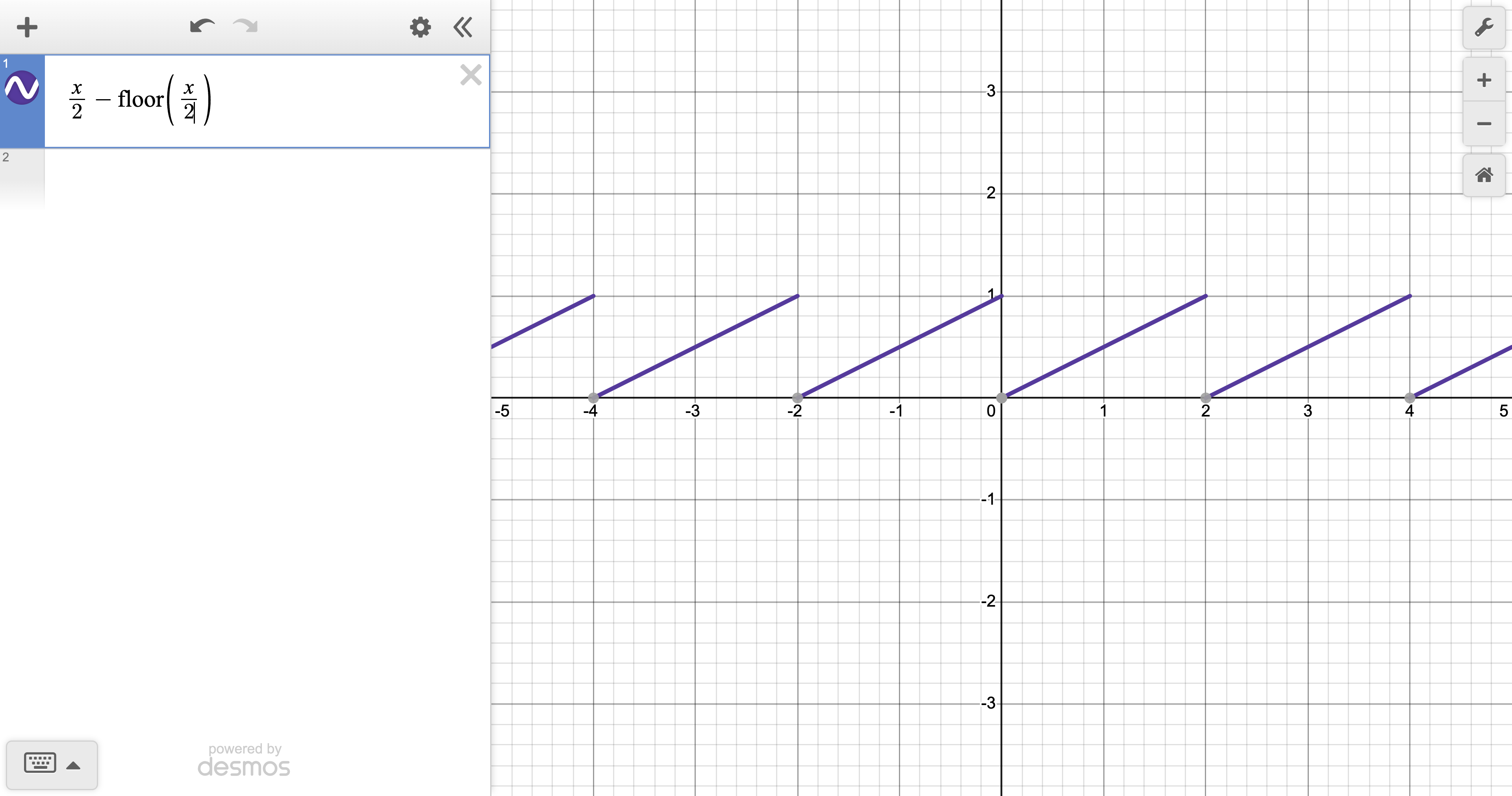
Exercise 5. Find the formula for a function whose graph looks like this, again using the floor function ‘$\lfloor \cdot \rfloor$’ as a building block:

We would like to argue the correctness of the following two-step process (divide the input by $2$, apply the function from Exercise 4):

Indeed, the two graphs featured above differ only by a horizontal dilation; dividing the input by $2$ “undoes” the dilation, at which point it suffices to apply the function pictured in the second graph; having declared our method correct, the answer is thus... $$ {x/2 - \lfloor x/2 \rfloor} $$ ...as obtained by “sticking” $x/2$ (the halved input) in place of “$x$” in “$\,x - \lfloor x \rfloor$”, the formula for the function from Exercise 4.
Note 1. One can check the answer by typing “x/2 - floor(x/2)” in DESMOS. Viz:
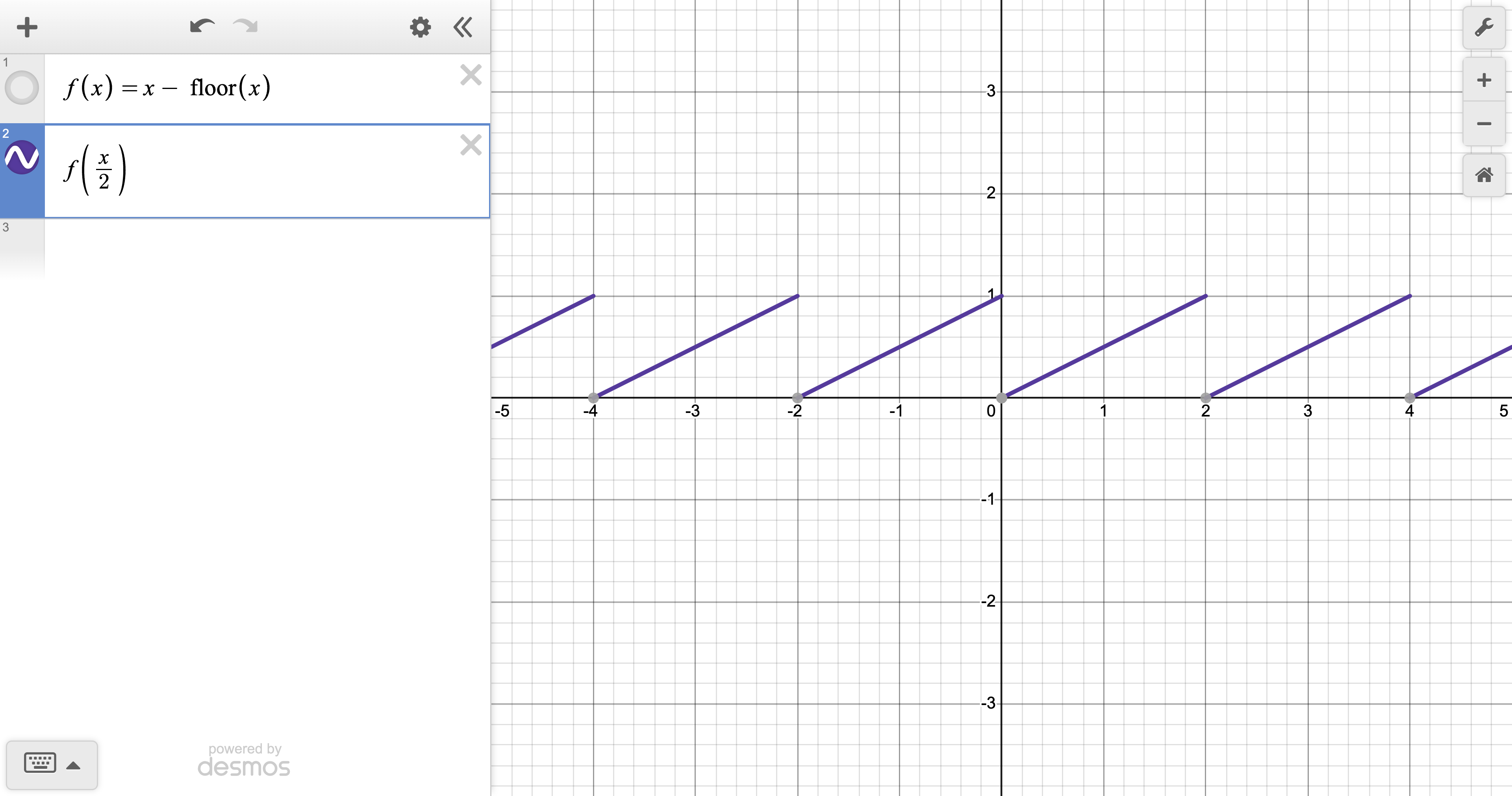
Note 2. Alternately, enter “f(x) = x - floor(x)” and then “f(x/2)”, viz:
Or we can be even fancier:
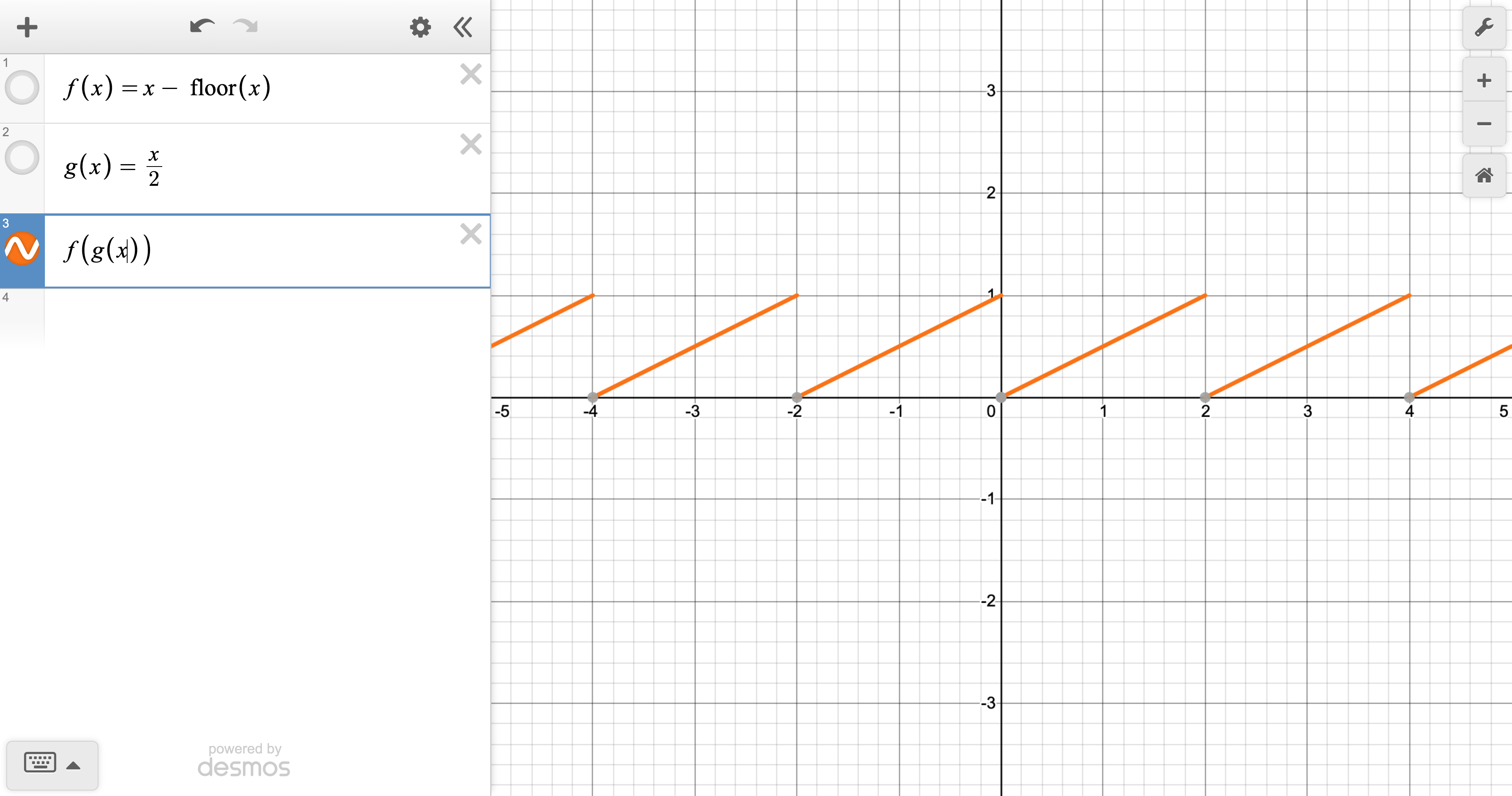
What you see above (the graph in orange) is the so-called
composition
of the functions $\Rule{0.12em}{0.8pt}{-0.8pt}f$ and $g$; in more detail, if we switch the “input tube” and “output tube” sides of a function...

...(compared to the drawing at the top of the chapter), then the composition of $\Rule{0.12em}{0.8pt}{-0.8pt}f$ and $g$, written $$ {\Rule{0.12em}{0.8pt}{-0.8pt}f \circ g} $$ and read
“$f$ of $\!\hspace{0.1em}{}g$”
(mathematicians have to invent a notation for everything—that little circle “$\circ$” is called the composition operator, by the way) is the function that you get by gluing $g$'s box to the right of $\Rule{0.12em}{0.8pt}{-0.8pt}f$'s box, like so:

In other words, $g$'s output is passed on to $\Rule{0.12em}{0.8pt}{-0.8pt}f$ for further processing. (A certain movie called “The Human Centipede” comes to mind.)
(To be perfectly clear,

$f \circ g$ is a function, defined as the above assemblage of “$g$ first, $f$ second”.)
Note 3. For a formal definition of “$f \circ g$”—something not based on pictures—one need only specify what $f \circ g$ does to inputs. Specifically: $$ \,{(f \circ g)(x) = f(g(x))}. $$ (So that equation is a formal definition.) One can also clarify that $$ {\text{dom}\, f \circ g = \{x\, \in\, \text{dom}\, g:\, g(x)\, \in\, \text{dom}\, f\}} $$ which is to say that the domain of $f \circ g$ consists of all $x$ such that: (i) $g(x)$ exists (a.k.a, “$x \in \text{dom}\, g$”) and, (ii) $f(g(x))$ exists (a.k.a., “$g(x) \in \text{dom}\, f$”).
Note 4. Amusingly—or not—both sides of $$ {(f \circ g)(x) = f(g(x))} $$ are read
“$f$ of $\!\hspace{0.1em}{}g$ of $x\hspace{0.1em}$”
since “$f \circ g$” is read “$f$ of $g\hspace{0.1em}$”, and “$f(\dots)$” is read “$f$ of ...”.
Exercise 6. Find formulas for functions whose graphs look like these:

For the first graph,
the
an
answer is
$$
2 \cdot(x/2 - \lfloor x/2 \rfloor)
$$
which simplifies to
$$
x - 2\lfloor x/2 \rfloor
$$
because all we have to do is to multiply
Exercise 5's formula by $2$.
For the second graph,
the
an answer is
$$
x/3 - \lfloor x/3 \rfloor
$$
because the problem is similar to Exercise 5 except with a
factor $3$ horizontal dilation.
For the third graph, we will first stop to find a formula for the function depicted here:

And that formula is...

...iiiiiiiS... $$ (x-1)/3 - \lfloor (x-1)/3 \rfloor $$ as obtained by substituting “$x - 1$” (the input, minus $1$) in place of “$x$” in “$\,x/3 - \lfloor x/3 \rfloor$”, the formula for the second graph. Then we multiply that by $3$ (to go from “” to “”, namely), meaning that the final answer is $$ 3 \cdot ((x-1)/3 - \lfloor (x-1)/3 \rfloor) $$ or $$ (x - 1) - 3\lfloor (x-1)/3 \rfloor $$ after simplification. (Or just $$ x - 1 - 3\lfloor (x-1)/3 \rfloor $$
though we personally prefer the previous form, it being more “talkative”.)
Exercise 7. If $$ \cos \!\hspace{0.1em}\mathrel{\raise.13ex{\substack{\small \circ \\ \small \circ}}} \mathbb{R} \rightarrow \mathbb{R} $$ (the “hollow dot colon” means that $\text{dom}\, \cos = \mathbb{R}$) is a function whose graph looks like so...

...then does the function... $$ {x \rightarrow \cos(1000x)} $$ ...have a graph that looks like a bunch of very tight bumps, or, instead, very flat & spaced-out bumps??
Consider how to “read off” a value of $y = \cos(1000x)$ from the graph $y = \cos(x)$:

By the first step, a
horizontal dilation by a factor 1000
maps the first graph onto the second graph—i.e., a point $$ (x, y) $$
is on the first graph if and only the dilated point $$ (1000x, y) $$ is on the second graph. The first graph is therefore some very compressed thing, full of scrunched bumps!
Note 1. One can also reason that a small change in $x$ results in a large change in ${1000x}$, so that ${\cos(1000x)}$ must “cycle” much faster through values than ${\cos(x)}$ does.
Exercise 8. Rewrite
without using “$\circ$”, using only the “definitional equation of function composition”, which is namely
(where $r$ and $s$ are functions); plz note that you will have to apply (**) twice, as each application of (**) makes one copy of the symbol “$\circ$” disappear, and (*) contains two copies of “$\circ$”!!

...which already constitutes progress towards our goal, since only one copy of “$\circ$” exists on the right-hand side! But
by the “definitional equation” again, so
...and this completes the computation!
Note 1. We can collect both steps of the computation into a single string of equalities:

Exercise 9. Same question as Exercise 17, but for “$f \circ (g \circ h)$” instead of “$(f \circ g) \circ h$”.
We will again evaluate the “outer” composition operator first and the “inner” composition operator second, where the “outer” composition operator is the one that is fewer pairs of parentheses away from the outside world:

So the first step is...
...by setting $r = f \circ g$, $s = h$ in the definitional equation, and the second step is...
...by setting $r = f$, $s = g$, and while replacing “$x$” by “$h(x)$”.
Note 1. The fact that $$(f \circ (g \circ h))(x)$$ and $$((f \circ g) \circ h)(x)$$ both evaluate to $$f(g(h(x)))$$ actually implies that $$f \circ (g \circ h)$$ and $$(f \circ g) \circ h$$ are the same function; this function is namely the function that maps $x$ to $f(g(h(x)))$ for all $x$ (or $$x \rightarrow f(g(h(x)))$$ in lambda notation).
Note 2. Because of this, we can write $$f \circ g \circ h$$ without any parentheses. (The point is: either way you parenthesize it you obtain the same function, so why bother?)
Note 3. The fact that
for all numbers $a$, $b$, $c$ is known as the
associativity
of addition; likewise, the fact that
for all numbers $a$, $b$, $c$ is known as the
associativity
of multiplication; and again likewise, the fact that
for all functions $f$, $g$, $h$ is known as the

associativity
of function composition.
Note 4. One of the best ways to explain & understand the associativity of function composition uses this picture:

In the above $A$, $B$, $C$, $D$ are sets while the arrows encode functions $f$, $g$ and $h$ that, respectively in reverse order, go from $D$ to $C$, $C$ to $B$, and $B$ to $A$. For example,
${\Large h(}$${\Large{}) =\hspace{0.2em}}$
because the arrow that originates at in set $D$ lands at in set $C$, and
${\Large g(h(}$${\Large{})){}=\hspace{0.2em}}$
because, pursuing that path onwards, the arrow that originates at in set $C$ lands at in set $B$, etc.
Under this representation one can “compute” $f \circ g \circ h$ by gluing arrows end-to-end. First, say, obliviate set $C$ in the middle right, then do the same with set $B$ in the middle left:

We can also get rid of $B$ first, $C$ second:

The first order of computation corresponds to the parenthetization “$f \circ (g \circ h)$” while the second corresponds to the parenthetization “$(f \circ g) \circ h$”. Intuitively, the reason they come out the same (in “step 6”, bottom left) is because each final arrow in the last diagram comes from a path-of-arrows in the original diagram, and the order in which the waypoints along a path are “straightened” (or “collapsed”) does not affect the origin point or destination point of the final arrow.
Note 5. The last series of diagrams might leave one with the impression that the composition of two or more functions can be “precomputed” by looking ahead along the path of yellow arrows. Just so you know, computers do not generically do this. For reason, computers are not given functions as tables of input-output values to know by heart but rather as “recipes” (synonyms: algorithms, code, programs) that allow them to compute an output for any given input. Moreover, there is no general way of flattening two recipes into a single, shorter one—when composing two functions the computer has, in general, no choice but to diligently apply each recipe in order—the first function first, the second function second.
Note 6. We have taken for granted the fact that two functions $f$ and $g$
are “equal” if and only if
they produce the same outupt for every input
but this is a actually subtle thing that has to do
with how functions are defined “under the hood”. Specifically,
mathematicians view functions as
long
lists of
sets of ordered pairs; for example—conceptual cold water shock ahead—
because VX-11/78A maps $0$ to $3.5$ and maps $1$ to $2.5$. (The presence of an ordered pair
means that input $a$ produces output $b$.) So two functions are equal if and only if they are equal
as sets of ordered pairs
because the set of ordered pairs is the underlying “thing”
that the function is. In particular, there is no notion of a
“formula” or of a “procedure” being attached to a function,
that might cause two functions to be considered unequal even if
they produce the same output on every input—producing the same
output on every input implies that the
list of
set
of ordered pairs is equal, and, perforce, that the two functions
are equal!!
Exercise 10. Show that $$ x^2 + 10x + 30 $$ can be written in the form $$ (x + \dots)^2 + \,\dots $$ for some numbers “$\dots$” and “$\dots$”.
The answer is $$ (x + 5)^2 + 5 $$ because $$ \begin{align} \,\,\,\,(x + 5)^2 &= x^2 + (2\cdot 5)x + 5^2 \\ &= \rule{0pt}{1.4em} x^2 + 10x + 25 \end{align} $$ and adding $5$ gives $x^2 + 10x + 30$.
Exercise 11. Solve Exercise 10 using algebra & variables.
Put an unknown “$U$” for the first set of dots and an unknown “$V$” for the second set of dots. Then $$ (x + U)^2 + V = x^2 + 10x + 30 $$ becomes the equation to satisfy. Expanding the left-hand side, we get: $$ x^2 + 2Ux + U^2 + V = x^2 + 10x + 30. $$ In order for this equation to hold as an equality between polynomials (i.e., for all $x$) the coefficients of $x^2$ on both sides of the equation must be equal, the coefficients of $x$ on both sides of the equation must be equal, and the constant terms on boths of the equation must be equal—this gives us $$ 1 = 1 $$ (equating the coefficients of $x^2$), and $$ 2U = 10 $$ (equating the coefficients of $x$), and $$ U^2 + V = 30 $$ (equating the constant terms). Only the latter two equations contain information. In particular, $$ 2U = 10 $$ implies $U = 5$, so $U^2 + V = 30$ becomes $25 + V = 30$, and $V = 30 - 25 = 5$. So $U = V = 5$, as previously found. (But now we know that the solution is unique, because the only number $U$ that satisfies $$ 2U = 10 $$ is $U = 5$, and the only number $V$ that satisfies $$ 25 + V = 30 $$ is $V = 5$.)
Exercise 12. Show that $$ x^2 + 10x + 30 = 0 $$ (cf$.$ Exercise 21) has no solutions $x \in \mathbb{R}$.
The equation is equivalent to $$ (x + 5)^2 + 5 = 0 $$ by Exercise 21, but this implies $$ (x + 5)^2 = -5 $$ which is an equation with no solution over the reals because the square of a real number is nonnegative.
Exercise 13. Show that $$ x^2 + 10x - 30 = 0 $$ has two solutions $x \in \mathbb{R}$.
The equation can be written $$ (x + 5)^2 - 55 = 0 $$ because $(x + 5)^2 = x^2 + 10x + 25$ and $25 - 55 = -30$. Passing $55$ to the other side, we find $$ (x + 5)^2 = 55 $$ which holds if and only if $$ \,x + 5 = \pm\sqrt{55} $$ or $$ \,x = -5 \pm\sqrt{55} $$ constituting two distinct solutions.
Exercise 14. What sequence of geometric transformations (rotations, translations, scalings, etc) maps the curve $$ {y = x^2} $$ onto $$ {y = Ax^2 + Bx} $$ for constants $A$, $B$ such that $A \ne 0$?
Write $$ {Ax^2 + Bx} $$ as $$ {A\Big(x^2 + {B \over A}x\Big)} $$ and then write $$ {x^2 + {B \over A}x} $$ as $$ {\Big(x + {B \over 2A}\Big)^2 - {B^2 \over 4A^2}} $$ so that, altogether, $$ {Ax^2 + Bx} $$ is rewritten $$ {A\left[\Big(x + {B \over 2A}\Big)^2 - {B^2 \over 4A^2}\right]} $$ that can be seen as descending from $y = x^2$ in three steps: $$ {y = x^2} $$ $$ {\downarrow} $$ $$ {y = \,\Big(x + {B \over 2A}\Big)^2} $$ $$ {\downarrow} $$ $$ {y = \,\Big(x + {B \over 2A}\Big)^2 - {B^2 \over 4A^2}} $$ $$ {\downarrow} $$ $$ {y = A\left[\Big(x + {B \over 2A}\Big)^2 - {B^2 \over 4A^2}\right]}. $$
Three steps, three geometric transformations! The third step effects a
vertical scaling by $A$
i.e., vertically stretches the graph by a factor $A$, because we multiply the value of $y$ by $A$. The second step effects a
vertical translation by ${-{B^2 \over 4A^2}}$
i.e., lowers the height of the entire graph by ${B^2 \over 4A^2}$, because we add $-{B^2 \over 4A^2}$ to the value of $y$. The first step, on the other hand, is entirely different: it is a
preprocessing
step, in that we mess with the input (i.e., $x$), instead of adding on (or “multiplying on”) to the current value of $y$.
To understand how a preprocessing step affects the shape of a graph, note that, more generally, a graph of the form $$ {y = f(x + a)} $$ (for some constant $a$) “fetches” values on the graph $$ {y = f(x)} $$ by going $a$ units to the right. The larger $a$ is, thus, the further $$ {y = f(x + a)} $$ drifts off to the left. For example, $$ {y = f(x + 20)} $$ has value $f(0)$ at $x = -20$, and if you replace $20$ with something larger, that position (i.e., $x = -20$) drifts even further off to the left! In any case, the graph $y = f(x + a)$ is the
leftward
translate by $a$ units of $y = f(x)$ and, as a consequence, the first step effects a
leftward translation by ${B\over 2A}$
of the curve $y = x^2$, or
horizontal translation by $-{B\over 2A}$
more elegantly put. (The second formulation doesn't assume a particular orientation of the $x$-axis, that's why it's “more elegantly put”, in our opinion.)
To recapitulate, the three transformations are, in order:
1. horizontal translation by $-{B \over 2A}$
2. vertical translation by ${-{B^2 \over 4A^2}}$
3. vertical scaling by $A$
* * * *
Note 1. You could do the vertical translation before the horizontal translation, geometrically it comes out the same. That order of geometric transformations would correspond to the following sequence of algebraic transformations: $$ {y = x^2} $$ $$ {\downarrow} $$ $$ {y = x^2 - {B^2 \over 4A^2}} $$ $$ {\downarrow} $$ $$ {y = \,\Big(x + {B \over 2A}\Big)^2 - {B^2 \over 4A^2}} $$ $$ {\downarrow} $$ $$ {y = A\left[\Big(x + {B \over 2A}\Big)^2 - {B^2 \over 4A^2}\right]} $$ ...in which the second step is a preprocessing step. (I.e., a step that replaces “$x$” with something else.)
Exercise 15. Let $x_0 \in \mathbb{R}$, $y_0 \in \mathbb{R}$ and $a \in \mathbb{R}$ with $y_0 \geq 0$, $a \ne 0.$ If you apply these transformations...
1. vertical translation by $-y_0$
2. horizontal translation by $x_0$
3. vertical scaling by $a$
...to the curve $y = x^2$, what are the roots of the final curve that you obtain? (Nb: Roots are values of $x$ such that $y = 0$.)
Start by noting that the point $(\sqrt{y_0}, y_0)$ is on the curve $y = x^2$, as well as the point $(-\sqrt{y_0}, y_0)$, because $(\sqrt{y_0})^2 = (-\sqrt{y_0})^2 =$ $y_0;$ here is a sketch of the situation before anything happens:

After vertically translating by $-y_0$ the roots will therefore be at $x = \pm\sqrt{y_0}$:

Then after horizontally translating by $x_0$ the roots mosey over to $x = x_0\pm\sqrt{y_0}$:

Lastly, vertical scaling does not affect the position of the roots, because it stretches the graph about the $x$ axis (here $a \approx 1.7$):

So the roots are at: $x = x_0 \pm \sqrt{y_0}$. (Like we found them after the second step.)
Exercise 16. Use the results of the previous two exercises to find the value(s) of $x$ such that $Ax^2 + Bx = 0$ for constants $A$, $B$ such that $A \ne 0$.
Well, $$ Ax^2 + Bx = 0 $$ obviously has solution $x = 0$ to start with, so we don't need the previous exercises for one of the roots at least—actually, $$ Ax^2 + Bx = x(Ax + B) $$ so the equation is equivalent to $$ x(Ax + B) = 0 $$ and so one of the roots is $$ x = 0 $$ and the other root is the value of $x$ such that $$ Ax + B = 0 $$ which is $x = -B/A$. (In order for the product $$ x(Ax + B) $$ to be $0$ you either need the first term to be $0$, leading us to $x = 0$, or the second term to be $0$, leading us to $Ax + B = 0$—the product of two things is $0$ if and only if one of the two things is $0$.)
So the roots are $x = 0$ and $x = -B/A$.
To complete the problem as we were asked, however, we will use the fact that $y = Ax^2 + Bx$ is obtained from $y = x^2$ by the following sequence of transformations (cf. Exercise 14):
1. vertical translation by ${-{B^2 \over 4A^2}}$
2. horizontal translation by $-{B \over 2A}$
3. vertical scaling by $A$
(We put the vertical translation first.) By Exercise 15, the roots of $y = Ax^2 + Bx$ are thus at
which looks a little different than our previous result of $x = 0$ and $x = -B/A$ until you realize that $$ \pm \sqrt{B^2 \over 4A^2} = \pm {B \over 2A} $$ (because $$ \left({B \over 2A}\right)^{\!2} = {B^2 \over 4A^2} $$ and even though ${B\over 2A}$ could be negative, the “$\pm$” on either side of the equation means that the set of values on either side of the equation is the same), so that (*) becomes $$ x = -{B\over 2A} \pm {B \over 2A} $$ and, on the one hand, $$ -{B\over 2A} + {B \over 2A} = 0 $$ while, on the other hand, $$ -{B\over 2A} - {B \over 2A} = -{2B\over 2A} = -{B\over A} $$ so here too we find that the roots are $x = 0$ and $x = -B/A$. (It must be the right answer!)
Exercise 17. True or false ($f$ and $g$ are functions):
| i. | $f \circ g = (x \rightarrow f(g(x)))$ | iii. | $f \circ g = (x \rightarrow g(f(x)))$ |
| ii. | $g \circ f = (x \rightarrow f(g(x)))$ | iv. | $g \circ f = (x \rightarrow g(f(x)))$ |
The true statements are i, iv, because $f \circ g$ is the function that maps an input $x$ to $f(g(x))$, and symmetrically for $g \circ f$.
Exercise 18. If $f$ and $g$ are functions then we define (and not just us but people in general) $$ f + g $$ to be $$ t \rightarrow f(t) + g(t) $$ (use ‘$x$’ if you like), i.e., to be the function that applies $f$ and $g$ separately and then takes the sum, and we define $$ fg $$ to be $$ z \rightarrow f(z)g(z) $$ (use ‘$t$’ if you like, hehe), i.e., to be the function that applies $f$ and $g$ separately and then takes the product. (These definitions are similar to how we define $$ f \circ g $$ to be $$ u \rightarrow f(g(u)) $$ for the symbol “$\circ$”, except that now we are defining the sum and product of functions, instead of their composition, namely.)
Given these definitions, which of the following equalities hold, in general for all functions $f$, $g$ and $h$? $$f \circ (g + h) = (x \rightarrow f(g(x)) + f(h(x)))$$ $$f \circ (g + h) = (x \rightarrow f(g(x) + h(x)))$$ $$(g + h) \circ f = (x \rightarrow h(f(x)) + g(f(x)))$$ $$(g + h) \circ f = (x \rightarrow (g + h)(f(x)))$$
The first equality is false because the right-hand side is actually $$ (f \circ g) + (f \circ h) $$ not $f \circ (g + h)$; the second equality is true; the third equality is true even though you would expect the right-hand side to be written $$ (x \rightarrow g(f(x)) + h(f(x))) $$ with “$g$” and “$h$” switched (but addition is commutative, so it doesn't matter); the fourth equality is true: it is the definition of “$\circ$”.
Exercise 19. What sequence of geometric transformations of length no more than 3 maps $$ y = x^2 $$ onto $$ y = Ax^2 + Bx + C $$ for constants $A$, $B$, $C$ such that $A \ne 0$?
Write $$ { Ax^2 + Bx + C} $$ as $$ { A\Big(x^2 + {B \over A}x + {C\over A}}\Big) $$ and, similarly to Exercise 14, write $$ { x^2 + {B \over A}x} $$ as $$ { \Big(x + {B \over 2A}\Big)^2 - {B^2 \over 4A^2}} $$ so that, altogether, $Ax^2 + Bx + C$ becomes $$ { A\left[\Big(x + {B \over 2A}\Big)^2 - {B^2 \over 4A^2} + {C\over A}\right]} $$ or $$ { A\left[\Big(x + {B \over 2A}\Big)^2 - {B^2 - 4AC\over 4A^2}\right]} $$ by putting things on a common denominator. (We have endeavored to keep the minus sign out front of the common denominator fraction in order to maintain the most similarity with the term “$-{B^2\over 4A}$” of Exercise 14, that also has a minus sign out front.)
By direct analogy with Exercise 14, the three transformations are thus...
1. horizontal translation by $-{B \over 2A}$
2. vertical translation by ${-{B^2 - 4AC \over 4A^2}}$
3. vertical scaling by $A$
...or...
1. vertical translation by ${-{B^2 - 4AC \over 4A^2}}$
2. horizontal translation by $-{B \over 2A}$
3. vertical scaling by $A$
...if we put the vertical translation first.
Exercise 20. What are the roots (i.e., solutions) $x$ of $$ Ax^2 + Bx + C = 0 $$ for constants $A$, $B$, $C$ such that $A \ne 0$?
The curve $$ y = Ax^2 + Bx + C $$ is obtained from the curve $y = x^2$ by the following sequence of transformations (cf. Exercise 19):
1. vertical translation by ${-{B^2 - 4AC \over 4A^2}}$
2. horizontal translation by $-{B \over 2A}$
3. vertical scaling by $A$
~
On the one hand, if $$ {B^2 - 4AC \over 4A^2} < 0 $$ then $$ -{B^2 - 4AC \over 4A^2} > 0 $$ and the vertical translation is upward, the curve detaches from the $x$ axis never to see it again, and there are no roots!
On the other hand, if $$ {B^2 - 4AC \over 4A^2} \geq 0 $$ then the roots are given by $$ x = -{B \over 2A} \pm \sqrt{B^2 - 4AC \over 4A^2} $$ by Exercise 15. $\rightarrow$ ~The End~ $\leftarrow$
Note 1. In fact, $$ \pm\sqrt{B^2 - 4AC \over 4A^2} = \pm {\sqrt{B^2 - 4AC} \over 2A} $$ (square both sides of the equation—in general, $$ \pm E = \pm F $$ as one set of two values equalling another set of two values, if and only if $$ |E| = |F| $$ or $$ E^2 = F^2 $$ —so that's why we say “square both sides”), so the formula for the roots can also be written $$ x = -{B \over 2A} \pm {\sqrt{B^2 - 4AC} \over 2A} $$ or $$ x = {{-B \pm \sqrt{B^2 - 4AC}} \over 2A} $$ as briefly flashed by, e.g., in Chapter 1.
Note 2. If $$ {B^2 - 4AC \over 4A^2} < 0 $$ then $$ \sqrt{B^2 - 4AC \over 4A^2} $$ does not exist, alerting you to the absence of roots, if you try to use the first formula we gave. Also $$ {B^2 - 4AC \over 4A^2} < 0\iff B^2 - 4AC < 0 $$ because $4A^2 > 0$ for all $A \ne 0$, so the second set of formulas would alert you to the absence of roots in that case, as well.
Exercise 21. Summon your senses of extrapolation & imagination to evaluate this expression: $$ (f \rightarrow x \rightarrow h \rightarrow {f(x+h) - f(x)\over h})(x \rightarrow x^2)(5)(0.1) $$ (Hint: The answer is a specific real number.)
...in an expression such as... $$ (x \rightarrow x^3)(6) $$ ...we pair the $x$ with $6$...

...and $6$ becomes the value to use for $x$ in “$x^3$”:

...; in an expression such as... $$ (x \rightarrow y \rightarrow x^3y)(6) $$ ...we also pair the $x$ with $6$...

...and $6$ becomes the value to use for $x$ in “$y \rightarrow x^3y$”:

...(in this case the result is not a number, but a function—a function is a mathematical object like another, after all); in an expression such as... $$ (x \rightarrow y \rightarrow x^3y)(6)(8) $$ ...we pair the $x$ with $6$ and the $y$ with $8$...

...and $6$ and $8$ become respectively the values to use for $x$ and $y$ in “$x^3y$”:

...; now in an expression such as... $$ (f \rightarrow x \rightarrow h \rightarrow {f(x+h) - f(x)\over h})(x \rightarrow x^2)(5)(0.1) $$ ...we pair the $f$ with $x \rightarrow x^2$, the $x$ with $5$, and the $h$ with $0.1$...

...and $x \rightarrow x^2$, $5$ and $0.1$ become respectively the values to use for $f$, $x$ and $h$ in “${f(x + h) - f(x)\over h}$”:

...; evaluating... $$ {(x \rightarrow x^2)(5 + 0.1) - (x \rightarrow x^2)(5) \over 0.1} $$ ...we... $$ {(x \rightarrow x^2)(5.1) - (x \rightarrow x^2)(5) \over 0.1} $$ ...get... $$ {5.1^2 - 5^2 \over 0.1} $$ ...this... $$ {26.01 - 25 \over 0.1} $$ ...thiiis... $$ {1.01 \over 0.1} = 1.01 \times 10 = 10.1 $$ ...result! (The answer is: ten point one.)
Chapter 4: Derivatives

Definitions. The derivative of a function $$ f : \mathbb{R} \rightarrow \mathbb{R} $$ is a (new) function $$ f' : \mathbb{R} \rightarrow \mathbb{R} $$ that gives the slope of $f$ at each point. In other words $$ f'(a) $$ is the slope of the graph $y = f(x)$ at $x = a$. And—surprise!—each pair of graphs above is a pair of the form $y = f(x)$ [$=$ “before”], $y = f'(x)$ [$=$ “after”]. (Meaning, the “after” graph records the slope of the “before” graph.) E.g.:

Note that $f'\!$ (read “$f$ prime”) remains undefined where $y = f(x)$ has a sharp “corner” and no well-defined slope. By opposition, if there is a well-defined tangent line to $y = f(x)$ at $x = a$ the slope of this tangent line supplies the value of $f'(a)$:


In fact, we can succinctly describe the derivative by... $$ f'(a) = \text{[slope of tangent line to $y = f(x)$ at $x = a$]} $$ ...with theunderstanding that $f'(a)$ is undefined if a tangent line does not exist or if the tangent is vertical. But for one last asterisk—and speaking of the existence, or not, of the tangent—note that the endpoint of a curve does not count as having a tangent, and therefore leaves a missing value for the derivative:

(In other words, “half-tangents” do not actually count as tangents—just a definition, the way it is!)
Vocabulary. A function $f : \mathbb{R} \rightarrow \mathbb{R}$ is
differentiable
if $\text{dom}\,\,f' = \text{dom}\,\,f$. Also, if $a, b \in \mathbb{R}$, $a < b$, $f$ is
differentiable on $[a,b]$
if $[a,b] \subseteq \text{dom}\, \,f'$. Lastly, $f$ is
differentiable at $a$
if $a \in \text{dom}\,\,f'$.
Sketching a Derivative. Say that you would like to sketch the derivative of the “before” function from the last “before”/“after” pair above (the one with the closed endpoints):

One method is simply to eyeball the slope at a few points along the curve, plot these values and interpolate:


...voilà!
An alternate approach is to start by determining intervals on which the derivative is positive and negative, and then to interpolate via the largest (respectively, smallest) value of the derivative in each interval:


The result (at bottom right) is a charming “robosketch” of the true derivative! (Well, charming in our opinion, at least.)
Derivative of a constant function. A constant function is a function of the form $$ x \rightarrow B $$ for some $B \in \mathbb{R}$ independent of $x$. The graph of the constant function is the line $$ y = B $$ of slope $0$. So

because at each $x$-value you find a slope of $0$, when you look up (down?) at the graph.
If we refer to $$ x \rightarrow 0 $$ as the
zero function
we can summarize the situation by saying that
~ the derivative of a constant function
is the zero function ~
or, more shortly,
~ the derivative of a constant is zero ~
(the way people usually state it), or
~ the derivative of the constant function $y = b$
is the constant function $y = 0$ ~
more longly.
Derivative of an affine function. An affine function is a function of the form $$ x \rightarrow Ax + B $$ for constants $A$, $B \in \mathbb{R}$. The graph of $x \rightarrow Ax + B$ is a line of slope $A$, so

because the slope of a line of slope $A$ is $A$, no matter where you put yourself on the line. In particular, $B$ plays no role in the derivative! ($\,$Just like in the case of a constant function, the derivative leaves no trace of $B$'s value—and for the same reason that $B$ effects a vertical translation that does not change the slope of anything.)
In words:
~ the derivative of the affine function $y = ax + b$
is the constant function $y = a$ ~
Or, flexing our linguistic prowess a tad more:
~ the derivative of an affine function is the
coefficient of its linear term ~
(The “linear term” of $y = ax + b$ is $ax$, of coefficient $a$.)
Example 1. One has $$ (x \rightarrow 3x + 1)' = (x \rightarrow 3) $$ as per $$ (x \rightarrow Ax + B)' = (x \rightarrow A) $$ with $A = 3$, $B = 1$.
Example 2. One has $$ (x \rightarrow 12 - x)' = (x \rightarrow -1) $$ as per $$ (x \rightarrow Ax + B)' = (x \rightarrow A) $$ with $A = -1$, $B = 12$.
Units of the Derivative. If units are present, we have $$ %\text{$[\hspace{0.08em}\!\![\hspace{0.07em}\,y$ axis units for $\Rule{0.12em}{0.8pt}{-0.8pt}f'\,]\!\!\hspace{0.06em}]$} \,= \left[\frac{\text{$y$ axis units for $\Rule{0.12em}{0.8pt}{-0.8pt}f$}}{\text{$x$ axis units for $\Rule{0.12em}{0.8pt}{-0.8pt}f$}} \right] \text{$y$ axis units for $f'$} \,= {\text{$y$ axis units for $\Rule{0.12em}{0.8pt}{-0.8pt}f$} \over \text{$x$ axis units for $\Rule{0.12em}{0.8pt}{-0.8pt}f$}} $$ because a value output by $\Rule{0.12em}{0.8pt}{-0.8pt}f'$ is the slope of a tangent line attached to the graph $y = f(x)$, and $$ %\text{$[\hspace{0.08em}\!\![\hspace{0.07em}\,x$ axis units for $\Rule{0.12em}{0.8pt}{-0.8pt}f'\,\hspace{0.03em}]\!\!\hspace{0.06em}]$}\, = \hspace{0.02em}\,\text{$[\hspace{0.05em}\!\![\hspace{0.09em}\,x$ axis units for $\Rule{0.12em}{0.8pt}{-0.8pt}f\,\hspace{0.03em}]\!\!\hspace{0.06em}]$} \text{$x$ axis units for $f'$}\, = \hspace{0.02em}\,\text{$x$ axis units for $f$} $$ because an input for $\Rule{0.12em}{0.8pt}{-0.8pt}f'$ is, originally, an input for $\Rule{0.12em}{0.8pt}{-0.8pt}f$.
For example, if the “before” graph has units of...
- seconds on the $x$ axis, meters on the $y$ axis

...then the “after” graph will have units of...
- seconds on the $x$ axis, meters per second on the $y$ axis
...while if the “before” graph has units of...
- years on the $x$ axis, dollars on the $y$ axis

...then the “after” graph will have units of...
- years on the $x$ axis, dollars per year on the $y$ axis
...and so on.
Units might additionally prompt us to refer to $f'$ as
the
rate of change
of $f$, or, depending, as the
instantaneous
rate of change of $f$. The latter bit of emphasis has to do with the fact that, in a general graph, the slope of the tangent keeps changing from point to point.
The second derivative. The second derivative of $f$ is the derivative of the derivative of $f$. It is written “$f''$”: $$ \,\,\,f'' = (f')'. $$ Likewise, we have, e.g., $$ \begin{align} \rule{0pt}{0.95em}f''' &= (f'')'\\ \rule{0pt}{1.25em}f'''' &= (f''')'\\ \rule{0pt}{1.25em}f''''{}\!\hspace{0.0691em}' &= (f'''')'\\ \end{align} $$ these being, namely, the third, fourth and fifth derivatives of $f$. One can also write $$ f^{(n)} $$ for the $n$-th derivative of $f$, so that, for example, $$ f^{(7)} $$ means the same as $$ f''''''' $$ but with the advantage that you don't have to squint and start re-counting the apostrophes several times over.
Example 4. We have

because, firstly, $$ (x \rightarrow 3x + 1)' = (x \rightarrow 3) $$ and, secondly, $$ (x \rightarrow 3)' = (x \rightarrow 0) $$ so that, from start to finish, $$ (x \rightarrow 3x + 1)'' = ((x \rightarrow 3x + 1)')' = (x \rightarrow 3)' = (x \rightarrow 0) $$ where we unpeel the onion starting from the inside. (Physically difficult.)
Example 5. More generally, $$ \,\,\,(x \rightarrow ax + b)'' = (x \rightarrow 0) $$ for all $a, b \in \mathbb{R}$, by a similar computation; a.k.a.:

~ the second derivative of an affine function is zero ~
Geometric interpretation of the second derivative. The sign of the second derivative—whether it is positive or negative—indicates whether a graph is “bending upwards” or “bending downwards”. Upward-bending graphs have a positive second derivative, whereas downward-bending graphs have a negative second derivative:

Reason like this:
the second derivative is
“the rate of change of the rate of change”.
Sorry: “the rate of change of the slope”.
(Same difference.)
Ergo, if the second derivative is positive, the
slope is increasing; if the second derivative is
negative, the slope is decreasing.
Moreover, an
increasing
slope gives curves a “bending upwards” shape, while a
decreasing
slope gives curves a “bending downward” shape!
To emphasize, if the second derivative is some
LARGE POSITIVE NUMBER
then the slope is increasing at that rate, which could result in a sharp bend upwards in the graph (unless you are near vertical already—you can't see the difference between slope $100$ and slope $1000$ very well, at most scales—nor between $-1000$ and $-100$, for that matter).
Likewise, if the second derivative is some
LARGE NEGATIVE NUMBER
then the slope is decreasing at [the absolute value of] that rate, which could result in a sharp bend downwards in the graph (unless you are near vertical already, once again, because verticality can disguise the presence of a significant change in slope, once again).
Vocabulary #1. Curves with increasing (technically: nondecreasing) slope are called convex, while curves with decreasing (technically: nonincreasing) slope are called concave. Viz:

Vocabulary #2. An inflection point is a point at the interface between convex and concave sections of a graph:

Example 6. The fact that $$ (x \rightarrow 3x + 1)'' = (x \rightarrow 0) $$ indicates that the graph $$ y = 3x + 1 $$ is neither “bending upwards” nor “bending downwards”—$0$ is neither positive, nor negative.
The Second Derivative of Position. A graph of the form...

...describes position as a function of time (look at the units); the derivative...


...describes velocity as a function of time; finally, the second derivative...


...describes
the rate of change of velocity
also known as the
acceleration
as a function of time.
Note that the units on the $y$ axis of the second derivative are given by $$ {\text{$y$ axis units for $f'$} \over \text{$x$ axis units for $f'$}} = {\text{m}/\text{s} \over \text{s}} = {\text{m} \over \hspace{0.1em}\text{s}\!{\,}^2} $$ because $f'' = (f')'$. The point is, a tangent tothe graph $y = f'(t)$ has a “rise” measured in meters per second and a “run” measured in seconds:

The ratio “rise over run” has the form $$ %\left[{\text{m}/\text{s} \over \text{s}}\right] %= \left[{\text{m} \over \text{s}} \right] \times \left[{1 \over \text{s}}\right] %= \left[{\text{m} \over \text{s}\!{\,}^2} \right] {\text{m}/\text{s} \over \text{s}} = {\text{m} \over \text{s}} \times {1 \over \text{s}} = {\text{m} \over \text{s}\!{\,}^2} %= {\text{m}/\text{s}\!{\,}^2} $$ which produces the above-mentioned units of the second derivative. Also note that a ratio of the form $$ \frac{\text{difference in velocity}}{\text{amount of time}} $$ is, indeed, an acceleration, in that acceleration is defined as “the increase in velocity per unit time”.
To summarize:
~ velocity is the derivative of position ~
~ acceleration is the derivative of velocity ~
* * *
Note. The exotic units $$ %\left[{\text{m} \over \,\text{s}\!{\,}^2}\right] {\text{m} \over \,\text{s}\!{\,}^2} %\text{m}/\text{s}\!{\,}^2 $$ can be read
meters per second squared
which sounds pretty cryptic, unfortunately, or
meters per second per second
which is better, or (slight difference!)
meters per second, per second
which is even better because it “shows” acceleration to be a number of m$/$s per second. (Acceleration is a number of m$/$s per second, no?)
Example 8. Over a period of $10$s, an object that is accelerating at a constant rate of $$ 2{\text{m}/\text{s}\!{\,}^2} $$ increases its velocity by

according to the template
$$ (\text{rate of change}) \times \text{(amount of time)}\\ = \text{(amount of change)} $$ or, more specifically,
$$ (\text{acceleration}) \times (\text{amount of time}) =\\ (\text{change in velocity}) $$
since acceleration is the rate of change of velocity.
The Jerk. The rate of change of acceleration has a name as well, being known as the
jerk
in physics. The units of jerk (or “the” units of jerk, since any units of same dimension would do as well) are $$ {\text{m} \over \,\text{s}\!{\,}^3} $$ or
meters per second, per second, per second
which is mildly amusing. Basically, the jerk specifies how many meters per second, per second (a measure of acceleration!) is being gained or lost per second.
The word “jerk” is aptly chosen, too, considering that people don't lose balance under constant acceleration, but, rather, when some some jerk occurs in the movement of their train or subway car, etc. What we are trying to say is that
constant acceleration
and
zero jerk
are synonymous, insofar as the everyday world is concerned—which is good, because these notions are also equivalent in the mathematical realm, what with jerk being the derivative of acceleration!
Postscript: Sums, Products, Quotients, and Differences of Functions. Coming briefly back to Chapter 3-related matters, if $$ f, g : \mathbb{R} \rightarrow \mathbb{R} $$ then $$ f \circ g = (x \rightarrow f(g(x))) $$ $$ f + g = (x \rightarrow f(x) + g(x)) $$ $$ fg = (x \rightarrow f(x)g (x)) $$ $$ %{f\over g} = (x \rightarrow {f(x) \over g(x)}) {f/g} = (x \rightarrow {f(x)/g(x)}) $$ $$ f - g = (x \rightarrow f(x) - g(x)) $$ with each equation being a definition. The notation $$ f \circ g $$ goes back to Exercise 5 of Chapter 3, with the little circle “$\circ$” being known as the composition operator, while the sum $$ f + g $$ and product $$ fg $$ of functions already appear in Exercise 18 of Chapter 3, also. On the other hand, the
quotient
(i.e., $f/g$) and
difference
(i.e., $f - g$) of two functions from $\mathbb{R}$ to $\mathbb{R}$ appear here for the first time! (We are “completing our collection”.)
Exercise 1. Sketch the derivative of a function with the following graph (what looks like a sharp corner is a sharp corner):

That would be:

(The derivative is $1/2$ when the slope is $1/2$, is $-1/2$ when the slope is $-1/2$, and is undefined at the corners.)
Exercise 2. Would the derivative of $$ y = {1\over x} $$ be a very large negative number, or a very large positive number, near $x = 0$? Or would it depend on which side of 0 you are?
The graph of $y = {1 \over x}$ looks like so:

As one can see, the slope is very negative near $x = 0$, on either side. So the answer is: “very large negative”.
Exercise 3. Sketch the
second
derivative of the graph in Exercise 1.
The second derivative is zero wherever the first derivative is flat, and is undefined wherever the first derivative is undefined; this gives the second derivative the following pockmarked appearance:

Note 1. Taking even further derivatives produces the same graph back, over and over again.
Note 2. “first derivative” is a synonym of “derivative”.
Exercise 4. If we pretend that the graph of Exercise 1 depicts the
distance that a car has traveled as a function of time,
position of a car as a function of time,
with hours (hr) on the $x$-axis and kilometers (km) on the $y$-axis,
what do the units become
on the axes of the first and second derivatives?
The units on the $y$ axis become kilometers, kilometers per hour, and kilometers per hours squared (or “kilometers per hour, per hour”), including the first graph. (Each time another derivative is taken, divide the units of the $y$ axis by the units of the $x$ axis.) These are the position, velocity, and acceleration of the car as a function of time:


Exercise 5. Is the following equation correct, incorrect, or nonsensical? $$ (x \rightarrow x + 1) \,+\, (u \rightarrow 2u + 1) \,=\, (t \rightarrow 3t + 2) $$
The equation is true! Syntactically, $$ (x \rightarrow x + 1) \,+\, (u \rightarrow 2u + 1) $$ is a
sum of functions
because $x \rightarrow x + 1$ and $u \rightarrow 2u + 1$ are both functions. Now by definition, the sum $$ f + g $$ of functions $f$ and $g$ is the function $$ x \rightarrow f(x) + g(x) $$ that maps a number to the sum of the individual values of the functions. So—for example— $$ \begin{align} & \,\,\,((x \rightarrow x + 1) \,+\, (u \rightarrow 2u + 1))(5) \\ =& \,\,\,(x \rightarrow x + 1)(5) + (u \rightarrow 2u + 1)(5) \rule{0pt}{1.5em} \\ =& \,\,\,(5 + 1) + (2\cdot 5 + 1) \rule{0pt}{1.5em} \\ =& \,\,\,3\cdot 5 + 2 = 17 \rule{0pt}{1.5em} \end{align} $$ and—with a general input $t$— $$ \begin{align} & \,\,\,((x \rightarrow x + 1) \,+\, (u \rightarrow 2u + 1))(t) \\ =& \,\,\,(x \rightarrow x + 1)(t) + (u \rightarrow 2u + 1)(t) \rule{0pt}{1.5em} \\ =& \,\,\,(t + 1) + (2t + 1) \rule{0pt}{1.5em} \\ =& \,\,\,3t + 2 \rule{0pt}{1.5em} \end{align} $$ which implies that, indeed, $$ (x \rightarrow x + 1) \,+\, (u \rightarrow 2u + 1) $$ is the function that maps each real number $t$ to $3t + 2$, i.e., is equal to the function $t \rightarrow 3t + 2$. (!!)
Note 1. One can also do the main computation with $x$ in place of $t$: $$ \begin{align} & \,\,\,((x \rightarrow x + 1) \,+\, (u \rightarrow 2u + 1))(x) \\ =& \,\,\,(x \rightarrow x + 1)(x) + (u \rightarrow 2u + 1)(x) \rule{0pt}{1.5em} \\ =& \,\,\,(x + 1) + (2x + 1) \rule{0pt}{1.5em} \\ =& \,\,\,3x + 2 \rule{0pt}{1.5em} \end{align} $$ Here we have two different $x$'s: the $x$ that denotes the input, and the $x$ that is used as a placeholder to describe how the first function acts.
Exercise 6. Complete the missing units for each strip below, based on those units that are given:

The pattern to respect is that, each time you take a derivative, the units on the $x$ axis stay the same, while the units on the $y$ axis become divided by those on the $x$ axis. This gives the unique solutions:

Note 1. A unit of “$1$” is a
dimensionless
unit. Dimensionless units arise when quantities are divided by like quantities. Think of dimensionless quantities as “pure fractions” or “pure ratios”. (Percentages are dimensionless—in fact the term
percentage
is synonymous with
dimensionless ratio
though if you spoke to people about “dimensionless ratios” they would look at you funny. Also percentages are a system of notation, whereby the symbol “%” means “divide the preceding number by 100, in order to discover the numerical value of the ratio I'm talking about”.) (To drive it home: In Chinese, the written expressions “$23\%$” and “$23/100$” are indistinguishable when read out loud; they are both read “$23$ over $100$”; that is the simple & correct way!)
Exercise 7. Among the functions below, which is the zeroth, first, and second derivative? (I.e., which is $f$, $f'$, and $f''$, assuming that relationship exists.)

The graphs are already in the right order: if “$f$” is the original function then $f$ is on the left, $f'$ is in the middle, and $f''$ is on the right:

For example, the graph on the left has a slope that starts at $\sim\!-1$ and ends at $\sim\!1$, while those are the values at which the graph in the middle starts and ends (and not coincidentally, since the graph in the middle is the derivative of the graph on the left!):

Moreover the middle graph has slope close to $0$ at either end, and some slope near $1.5$ or $2$ towards the middle, matching the values of the graph on the right:


(Taking one more derivative would produce a zigzag, by the way.)
Exercise 8. Given these graphs...

...what can you say about $g'(x)$? (Produce the best sketch of $g'(x)$ that you can, taking into account all the information above.) (Don't get us wrong: You don't need the second derivative to sketch the first derivative, but if you're a human and not a machine, it can help!)
To start with, the slope of $g$ seems to be about $-1.5$, $0$ and (a bit greater than) $2$ at $x = -2$, $x = 0$ and $x = 2$ respectively:

This already gives us three points from which to interpolate a basic approximation to the graph $y = g'(x)$:

But the graph of $g''(x)$ indicates more, namely that $g'(x)$ has a slope that rises from $\approx 0.2$ near the left edge of the graph up to $1.3$ at $x = 0.5$, before falling again to $0.6$ past $x = 2$:

As a second step, we thus “bend into shape” our previous sketch to produce these slopes...

...achieving our final answer.
Note 1. For reference, the actual derivative looks like so:

Exercise 9. Given these graphs...

...sketch $y = h'(x)$, analogously to Exercise 10.
Firstly, the graph of $h(x)$ seems to have slope $0$ around $x = 0.6$...

...which gives us one data point on the curve $y = h'(x)$ to start with...

...moreover, by the graph of $h''(x)$, the slope of $h'(x)$ is near $-1/3$ on an interval that is approximately (say) $[-0.85,0.7]$....

...so, as a second step, we can extend the graph of $h'(x)$ by a segment of slope $-1/3$ on this interval:


(To achieve a passable slope of $-1/3$ we modeled ourselves on a nearby grid segment.) Next, $h(x)$ has slope $\approx 1.2$ at $x = -2$, and slope $\approx -0.9$ (?) at $x = 2$:

This gives us two more points on the graph $y = h'(x)$:

Then, because the second derivative has value $\approx -1/3$ for $x \leq -1.6$ (about) and for $x \geq 1.5$ (about)...

...we extend these two new data points by segments of slope $-1/3$...

...on the relevant intervals. (I.e., for $x \leq -1.6$ and for $x \geq 1.5$.) The last step is to join the existing segments by some kind of “connector curves” of yet-to-be-determined shape:

Since $h''(x)$ shows that the two connectors have slopes of about $-1/3$ at their edges and slopes of about $-1.4$ and $-1.6$ (respectively) near their middles...

...our final answer, given by the following sketch, is obtained by “bending into shape” the connector curves...

...to give them a slope of $-1/3$ at their endpoints, and slopes of $-1.4$, $-1.6$, respectively, in their middles.
Note 1. Here is the actual graph of $h'$:

Exercise 10. If you scale the graph of a function $f$ vertically by a factor $2$—i.e., multiply each output by $2$—is the derivative also scaled by $2$?
Yes, this is the case. For a joke way of seeing it, here is a graph of a putative function $f$, before and after scaling:

The second graph truly is the first graph vertically scaled by a factor $2$, because the scale on the $y$ axis has been doubled. This means that the ratio $$ {\text{rise}\over \text{run}} $$ has doubled in the second graph, because “rise” has doubled (each $y$-coordinate is twice as large!), whereas “run” stays the same. (So the slope of the tangent has doubled, so the derivative is doubled.)
Exercise 11. Where is the rate of change of the function below, on the part shown, greatest? And where is the
rate of change of the rate of change
greatest?

The rate of change is the slope, which is greatest along the right-hand portion of the curve:

On the other hand,
the rate of change of the rate of change
[a.k.a., second derivative] is the rate of change of the slope, and that will be greatest at the first bend of the curve, where the slope is changing at the fastest rate:

(Well, believe us or not, but we're right!)
Exercise 12. In the following graph, which curve might be a derivative of which other curve?

As it happens—and by the exact method that we used to generate these curves—the blue is the derivative of the red:

Likewise, the derivative of the blue is the yellow, the derivative of the yellow is the green, and the derivative of the green is the red, at which point it starts all over again! (For example, the fifth derivative of the red curve is the blue, because the fourth derivative of the red curve is itself.)
Note 1. After all, the slope of these curves keeps oscillating between two fixed values—the “most slanted up” and the “most slanted down”—so their derivatives were always going to have an oscillatory pattern, as well.
Note 2. Because “most slanted up” occurs when the curve has not yet crested, but when the derivative is already in the process of cresting (that's why it's “most slanted up”), the derivative is ahead of the original curve by half a bump, not the other way around:

Note 3. When we examine the velocity of a particle moving in the plane, we examine the velocities of its shadow on the $x$- and $y$-axes:

The velocities of the two shadows encode the overall “two-dimensional” velocity of the particle. (No need for quotes, really: the velocity is two-dimensional.)
Here's another point of view: just like
position
is encoded by a pair of numbers—sometimes known as the position vector by the way, where “vector” is a term of art for “pair of numbers”—so the
velocity
is encoded by a pair of numbers—equally known as the velocity vector—which is no coincidence, because the first coordinate of the
velocity vector
is the derivative of the first coordinate of the
position vector
and likewise for the second coordinate—two coordinates, two rates of change!

Geometrically, if we use the $x$- and $y$-components $v_x$ and $v_y$ of the velocity to draw an arrow emanating from a point on the curve, this arrow is tangent to the curve, and the
length
of the arrow is the
speed
of the particle at that moment in time. More precisely, if you let the particle drift at the exact same $x$- and $y$-velocities $v_x$ and $v_y$ that you measured at the root of the arrow for one unit of time, the particle would cover exactly the length of the arrow in that one unit of time, no more no less, because the particle would cover $v_x$ units in $x$ and $v_y$ units in $y$. And speed being
distance per unit time
the length of the arrow is, therefore, the speed!
Now consider not one but four particles, going around a unit circle in clockwise fashion, 90° apart in phase, at unit speed (“unit speed” = speed 1, “unit circle” = radius 1) (ps: We center the circle at the origin):

The
position vectors
of the particles are as follows:

(You can't really see it so well, but each arrow originates at $(0, 0)$.) While the
velocity vectors
are as follows:

(Like the position vectors, the velocity vectors keep changing instant by instant—this is the subtlety of calculus!) The velocity vectors have length $1$ because the speed is $1$, & are brushed in the direction of travel.

(Nb: When we draw a vector as an arrow we mean that the first coordinate of the vector is equal to the horizontal displacement from the tail of the arrow to the head of the arrow, and likewise that the second coordinate is equal to the vertical displacement from the tail of the arrow to the head of the arrow.)
Due to the 90° rotations and uniform lengths of $1$, one particle's velocity vector is another particle's position vector; for example, the red particle's velocity vector is the blue particle's position vector:

Focusing on the $x$-coordinates, for example,
the velocity in $x$ of the red particle is
the position in $x$ of the blue particle
at any given moment in time. This also means:
the rate of change of the $x$-coordinate of the red particle is the $x$-coordinate of the blue particle
...because “velocity in $x$” is the same as “rate of change of the $x$-coordinate”.
Concretely, if you graph the $x$-coordinates of the red and blue particles on the same graph, the rate of change of the red particle's $x$-coordinate will equal the value of the blue particle's $x$-coordinate. These are the reds and blue curves from the problem statement, if we start the red particle at position $$ (1, 0) $$ at time $t = 0$:

If we add the $x$-coordinates of the green and yellow particles, we find the graph from the problem statement!
Note 4. If needed, here is an illustration of one $360^\circ$ rotation of the particles of Note 3, with each curve being an $x$-coordinate:

(If the above just looks like a confusing mess then don't sweat it—it's not that important.)
Note 5. Take a look at this figure again:
The derivative is
ahead
of the function—the values that you see now on the derivative are values you will see a little later on the function—because the blue particle is, likewise,
ahead
of the red particle, so that $x$-coordinates you see now on the blue particle will be seen a little later on the red particle! (In particular, if you wanted to generate the same curves with a counterclockwise rotation, you could do that, but you would have to reverse the order of the particles around the circle to keep the blue particle ahead of the red particle, the yellow particle ahead of the blue particle, etc.)
Exercise 13. How can we generate the following set of curves by rotating points around a circle, and tracking their $x$-coordinates? (This graph is an exact $2$$\times$ [“two x”] vertical dilation of the graph in Exercise 12.) Should we use a circle of radius $2$, or make the points go twice as fast? Or both? Or something else yet?

The values oscillate between $+2$ and $-2$, so we need a circle of radius $2$ to generate these curves. Also the values go through one cycle in the same amount of time as the particles of Exercise 12, but the circle has twice the circumference (having twice the radius), so the particles are going twice as fast! (I.e.: speed 2, since the particles of Exercise 12 have unit speed.)
Note 1. In this and in the previous exercise the units of time and distance are “anonymous”: distance could be meters, kilometers, or anything, and time could be seconds, hours, etc—it doesn't matter. However, one should be aware that what amounts to
unit speed
under one set of units is no longer “unit speed” under a different set of units—this is not a “physical” property of the particles, but, rather, a “mathematical” property that holds only for one specific “tweaking” of the units.
Exercise 14. Exercise 12 exhibits a function $f$—in fact, four different functions $f$—such that $$ f' \ne f $$ and $$ f'' \ne f $$ and $$ f''' \ne f $$ but $$ f^{(4)} = f $$ surprise, surprise! Can you do the same with “$5$” instead of “$4$”? I.e., find a function $f$ such that $$ f^{(n)} \ne f $$ for $n = 1, 2, 3, 4$ but $$ f^{(5)} = f $$ ...?
We can naïvely try to imitiate how the curves of Exercise 16 are generated by placing five equally spaced particles around the unit circle (“the” unit circle is the one centered at $(0, 0)$, by convention), instead of 4:

The idea would be that the
velocity vector
of the red particle is the
position vector
of the blue particle, likewise for the blue and yellow particles, and so on. (Position vectors shown above.) For example, at the instant above, the velocity vectors would be as follows:

The velocity vectors are
NOT
tangent to the unit circle, and so the particles will leave the circle! (But that's OK.) In one-tenth a unit of time, for example, the particles would travel approximately one-tenth their velocity vectors, that would bring them to approximately these new positions:

In the next one-tenth unit of time we can apply a similar approximation again, advancing the particles by ${1\over 10}$th of [the current approximation to] their velocity vectors. Skipping the construction lines:

Applying the same process for $8$ more steps:

To be clear, in the above figure, the position of the red particle at, say, the fifth step...

...is obtained by starting from the red particle's position at the fourth step...

...and adding one-tenth of the approximation that we have to the red particle's velocity vector at that moment, that approximation being namely the blue particle's position vector at the fourth step ($t = {4\over 10}$)...

...and we do the same for each particle, to advance to the next step.
If we stop $10$ times as often, advancing the clock by ${1\over 100}$th of a unit of time at each step, the same figure becomes just a blur (still going from $t = 0$ to $t = 1$):

To visualize such a fine-grained approximation we need to revert to drawing the particles as points. In the following figure the colored paths are points that come from a “${1\over 100}$th” approximation, while the orange dots are the old positions obtained from a “${1\over 10}$th” approximation:

Zooming in a bit (or else we still can't see anything):


In any case, even the “${1\over 100}$th” approximation is just an approximation, but the point is that such approximations do converge to a set of “true” particle paths, as pictured in Fig$.$ 1, that can be computed by some wizards; as time can be played forward or backward, these paths form doubly-infinite spirals—in to infinity, out to infinity.
In any case [take two] the point is that whether or not you are one of the wizards, you can
guess
the existence of these five paths—sort of “feel” that they exist! (This is a moral consolation prize, at least.)
We can also convert the paths into a function $$ f $$ that satisfies the problem requirements.
For example let $f$ be the function that, given a time $t$, outputs the $x$-coordinate of the red particle at $t$; then, to spell it all out, since
the rate of change of the $x$-coordinate of the red particle is the $x$-coordinate of the blue particle
$f'$ is the $x$-coordinate of the blue particle; and since
the rate of change of the $x$-coordinate of the blue particle is the $x$-coordinate of the yellow particle
$f''$ is the $x$-coordinate of the yellow particle; and since
the rate of change of the $x$-coordinate of the yellow particle is the $x$-coordinate of the green particle
$f'''$ is the $x$-coordinate of the green particle; and since
the rate of change of the $x$-coordinate of the green particle is the $x$-coordinate of the purple particle
$f''''$ is the $x$-coordinate of the purple particle; and since
the rate of change of the $x$-coordinate of the purple particle is the $x$-coordinate of the red particle
$f''''' = f^{(5)}$ equals $f$.
Note 1. If you graph the $x$-coordinates of the 5 particles over time, each in their color, you get a graph like so, in which blue is the derivative of red, yellow is the derivative of blue, etc; the function $f$ can be taken to be any one of these curves:

Note 2. There is nothing special about $x$-coordinates vis-à-vis $y$-coordinates. You can also define $f(t)$ to be, e.g., the $y$-coordinate of the red particle at time $t$.
Note 3. It is worth noting that, in fact, the $x$- and $y$-coordinates live separate lives. The rate of change of each $x$-coordinate is some other $x$-coordinate, and the rate of change of each $y$-coordinate is some other $y$-coordinate.
Note 4. Adding to this observation, we don't need to start the particles in a symmetric configuration. Symmetry only helps to picture how the positions of the particles will evolve without making any computations. We also don't need to work in two dimensions. We can place the particles in a one-dimensional world, e.g., ...

...(the initial positions really don't matter much, as long as you don't give all the particles the same initial position, or else you won't have $f \ne f'$ etc) and stipulate the same rules, namely that the
velocity
(now $1$-dimensional) of the red particle be the
position
(now $1$-dimensional) of the blue particle and so on—you can “release” the particles from their initial configuration and simulate (or compute exactly, if you have the know-how) their motion by the same methods as above. The five position functions obtained are each a solution $f$ to the problem. (But this solution will typically look more chaotic than the curves from Note 1.)
Note 5. In fact, our symmetric two-dimensional solution is an instance in which you can say that


the whole is simpler than the parts
in that you would never spot the symmetry at play, or have a chance of eyeballing the long-term evolution of the system, if you were shown just the $x$-coordinates, or just the $y$-coordinates, on their own!
Exercise 15. If we seek a function $f : \mathbb{R} \rightarrow \mathbb{R}$ such that $$ f^{(17)} = f $$ and such that $f \ne 0$ (or: $f \ne (x \rightarrow 0)$, pedantically) and such that $f$ grows relatively slowly in either the positive or negative direction of the number line, insofar as such things are concerned, what would our options be?
Take $17$ particles equally spaced out along the unit circle, such as these (shown here with position vectors):

Set the velocity of particle $$ {\Large 1} $$ equal to the position of particle $$ {\Large 5} $$ and keep going by this pattern, making the velocity of each particle equal to the position of the particle that is $4$ later; in the configuration above, the velocity vectors end up looking like so, for example:


Maintaining this relationship at all points in time, and given that the velocity vectors point very slightly outward from the unit circle, and because all the symmetry and all the angles are maintained as we play time forward or backward, the particles spiral gently outward/inward from the circle for time forward/backward, respectively. Taking $f(t)$ to be the $x$- or $y$-coordinate of any one of the particles (e.g., particle $1$) at time $t$ gives an oscillating function whose $17$th derivative is itself (because the rate of change of the $x$-coordinate of particle $1$ is the $x$-coordinate of particle $5$, etc, until we make it all the way back to particle $1$), and that grows comparatively slowly over time. ~The End~
Note 1. In case you're curious, the actual spiral paths of the particles look like so:

...and if you take the $x$-coordinates of
the particles over time, with time $t = 0$
corresponding to the original configuration
depicted where particle 1 is at $(1, 0)$, you
find
paths
functions that look like so:

For example, the derivative of curve , highlighted below in red, is curve , highlighted in blue:

...and taking sixteen more derivatives starting from curve we would go through curves , , , , ..., , before finally coming back to curve !
Note 2. It can be interesting to examine what goes wrong if we attempt to make the velocity vectors even more tangent to the unit circle. For example, if we start the particles so that particle 5 is at $90^\circ$ exactly from particle 1, particle 9 is at $90^\circ$ exactly from particle 5, and so on, until we reach particle 14, the last particle in this order; then we have the following starting configuration:

To parse the above figure, understand that:
- the red arrows indicate which particle takes its velocity from the position of which other particle; for example, particle 1 has velocity equal to the position of particle 5
- particles that occupy the same starting position on the unit circle appear stacked together, as a representation device; for example, particle 2 has the same starting position as particle 5
(Note that the red arrows have to form a cycle of length 17 in order for us to later extract a function $f$ such that $$ f^{(17)} = f $$ but this is the case: the red arrows only “close the loop” after going through all 17 particles!)
In this starting configuration, all velocity vectors are exactly tangent to the unit circle
EXCEPT
for particle 14, whose velocity vector, being the position of particle 1, is straight out from the circle! So, as we “start time”, particle 14 will push out from the circle, that will in turn affect particle 10, and so on, until all particles end up being “peeled off” from the circle, in due time; if you are so curious, the particle trajectories end up like so (shown only for $t \geq 0$):

The particles shoot of to infinity in short order—the solution is much worse—for fun we have also highlighted two particle trajectories in this figure:
- in blue, particle 1, the last particle to be (noticeably*) “peeled off” from the circle (*all particles are instantaneously peeled off from the circle to some degree, as one particle's slight deviation affects the next, that affects the next, etc)
- in red, particle 14, the first particle to leave the circle—but because its velocity vector is given by particle 1, which itself starts by going around in a circle, it, too, starts out by going around in a circle!
(The point is: if your velocity vector is tracing a circle centered at $(0, 0)$—at a uniform rate—then you, too, are going around in a circle—it's just that your circle could be centered anywhere, not necessarily at $(0, 0)$!)
Exercise 16. Add elements to the following drawing...

...such that it becomes a “complete” illustration of this here algebraic expression... $$ {f(x+h) - f(x) \over h} $$ ...and reveal the “geometric meaning” of the expression, if any.
This version pictures all the elements that appear in the fraction:

The point is: the fraction $$ {f(x + h) - f(x)\over h} $$ is seen to have the form rise over run, and is more precisely equal to the slope of the pale brown line going through the point

at one end, and

at the other end. (This is also the case if $h$ is negative, by the way.)
Note 1. A fraction of this form is called a Newton quotient.
Note 2. The pale brown line is sometimes known as the secant [through $(x, f(x))$, $(x+h, f(x+h))$]. “Secant” is a general term for “line passing through two specified points on another curve”.
Note 3. If we let $h$ drop to $0$, and if $f$ is differentiable at $x$, the Newton-quotient-a.k.a.-slope-of-the-secant approaches $$ f'(x) $$ because the secant approaches the tangent, in that case, and the slope of the secant is also, perforce, approaching the slope of the tangent, which is $f'(x)$. (But you cannot directly set $h = 0$, because $$ {f(x+0)-f(x)\over 0} = {0 \over 0} $$ is undefined.)
Exercise 17. In this exercise we consider two points in time $t_0$ and $t_0 + \Delta{}t$ (here “$\Delta{}t$”, read “delta $t$”, is a standard notation for a small amount of time):

We also consider quantities $A$ and $B$ that are changing with time; $A$ and $B$ have some value at $t_0$, and, say, grow to be larger at $t_0 + \Delta{}t$:

More specifically, we are interested in the change in the value of the product $$ \Large AB $$ over said course of time.
To introduce an unsolicited metaphor, imagine $A$ and $B$ as


that are crossing a hallway surveyed by a cat. One side of the hallway is time $t_0$, the other side of the hallway is time $t_0 + \Delta{}t$. So great is their terror that $A$ and $B$ have decided to scurry across the hallway one at a time. First $A$ will go, then $B$. In so, we can separate the following moments of interest (“moments” that exist inside the metaphorical timeline of the story, not on the $t$-number line, to be clear):
- when $A$ and $B$ are both still at $t_0$
- when $A$ has made it to $t_0 + \Delta{}t$, and $B$ is still at $t_0$
-
when $B$'s tail is sticking out of the cat's mouth, andwhen $A$ and $B$ have both made it to $t_0 + \Delta{}t$
Correspondingly, the product $$ \Large AB $$ changes in two increments: first as $A$ makes it to the other side of the hallway (and $A$ grows bigger); then as $B$ joins him/her (and $B$ grows bigger). In an equation:

If we divide the above equation by $\Delta{}t$ and let $\Delta{}t$ drop to $0$, what does each term become?
Dividing by $\Delta{}t$:

As $\Delta{}t$ approaches $0$, the term on the left-hand side approaches $$ (AB)'(t_0) $$ where we view $A$ and $B$ as functions of time with, therefore, the product $AB$ also becoming a function of time. (By definition, $AB$ is the function $$ t \rightarrow A(t)B(t) $$ where $A(t)$ is the value of $A$ at time $t$, $B(t)$ is the value of $B$ at time $t$.) Indeed, a ratio of the form $$ {f(t_0 + \Delta{}t) - f(t_0)\over \Delta{}t} $$ is a Newton quotient (cf. Exercise 16), that approaches $$ f'(t_0) $$ as $\Delta{}t$ approaches $0$, assuming $f$ is differentiable at $t_0$ (cf. Exercise 16 Note 3), and

has the form $$ {f(t_0 + \Delta{}t) - f(t_0)\over \Delta{}t} $$

for $f = AB$.

The first term on the right-hand side, for its part, approaches
$$ B(t_0)A'(t_0) $$ as $\Delta{}t$ approaches $0$. Indeed, when you write it out, that term becomes the algebraic expression
where every term on top contains a “$B(t_0)$”, that can therefore be factored out, giving us the equivalent expression $$ B(t_0)\cdot{A(t_0 + \Delta{}t) - A(t_0) \over \Delta{}t} $$ that, you will notice, has the form $$ B(t_0)\cdot{f(t_0 + \Delta{}t) - f(t_0) \over \Delta{}t} $$ for $f = A$, and thus approaches $$ B(t_0) \cdot A'(t_0) $$ as $\Delta t$ approaches $0$, by the property of the Newton quotient.

Lastly the most interesting term is the second term on the right-hand side! Symmetrically to the first term on the right-hand side, the second term approaches
$$ A(t_0)B'(t_0) $$ as $\Delta{}t$ approaches $0$, but the reasons are slightly different! (Slightly.) Indeed, this term, written out, is $$ {A(t_0 + \Delta{}t)B(t_0+\Delta{}t) - A(t_0+ \Delta{}t)B(t_0) \over \Delta{}t} $$ which is equal to $$ A(t_0 + \Delta{}t)\cdot{B(t_0+\Delta{}t) - B(t_0) \over \Delta{}t} $$ by factoring out the common term $A(t_0 + \Delta{}t)$; and $$ {B(t_0+\Delta{}t) - B(t_0) \over \Delta{}t} $$ approaches $$ B'(t_0) $$ as $\Delta{}t$ approaches $0$, like before (when we had $AB$ or $A$ instead of $B$) whereas $$ A(t_0 + \Delta{}t) $$ —which is a bit different from before—approaches $$ A(t_0) $$ as $\Delta{}t$ approaches $0$—so that makes up $A(t_0)B'(t_0)$. (The
differentiability
of $A$ and $B$ at $t_0$—that we are tacitly assuming—implies
continuity
as well, which implies that $A(t_0 + \Delta{}t)$ approaches $A(t_0)$ as $\Delta t$ approaches $0$.)
Summarizing, the three terms separately approach $$ (AB)'(t_0) $$ $$ B(t_0)A'(t_0) $$ $$ A(t_0)B'(t_0) $$ as $\Delta{}t$ approaches $0$ and, in fact, because the equation holds no matter how close we make each term to its respective limit above, one can conclude that $$ (AB)'(t_0) = B(t_0)A'(t_0) + A(t_0)B'(t_0) $$ for functions $A$, $B$ differentiable at a point $t_0$.
Nb: This result is known as the product rule.
Note 1. Keeping things alphabetical everywhere, the same equation is more often written $$ (AB)'(t_0) = A'(t_0)B(t_0) + A(t_0)B'(t_0) $$ with “$A'(t_0)B(t_0)$” in the middle. (But which is the same, of course, as $B(t_0)A'(t_0)$.)
Exercise 18. The identity $$ (f + g)' = f' + g' $$ happens to be true for differentiable functions $f$, $g$. What English-language aphorism can summarize it? (This identity is known as the sum rule, by the way.)
One can say
the derivative of the sum is the sum of the derivatives
or
the rate of change of the sum is the sum of the rates of change
or (we made this one up)
the rate of change of the aggregate is the sum of the rates of change of the components
(etc).
Exercise 19. If we rewrite the “product rule” of Exercise 17 in the same terse style as the “sum rule” of Exercise 19, what do we obtain?
The form of... $$ (fg)'(t_0) = f'(t_0)g(t_0) + f(t_0)g'(t_0) $$ ...that follows the style of... $$ (f + g)' = f' + g' $$ ...is... $$ (fg)' = f'g + fg' $$ ...this. (Valid for differentiable functions $f$, $g:$ $\mathbb{R} \rightarrow \mathbb{R}$.)
Note 1. Whereas $$ (fg)'(t_0) = f'(t_0)g(t_0) + f(t_0)g'(t_0) $$ is an equality between real numbers, $$ (fg)' = f'g + fg' $$ is an equality between functions. So there is a more-than-skin-deep difference between the two forms. Also note that each form has its own “qualitatively distinct” qualifying conditions.
(To wit, $$ (fg)'(t_0) = f'(t_0)g(t_0) + f(t_0)g'(t_0) $$ holds “for $t_0$ at which $f$ and $g$ are differentiable”, while $$ (fg)' = f'g + fg' $$ holds “for differentiable functions $f$, $g$”.)
Exercise 20. If the identities $$ (f + g)' = f' + g' $$ and $$ (fg)' = f'g + fg' $$ for differentiable $f$, $g$ are deemed “differentiation formulas”, then what is a third “differentiation formula” already encountered (in possibly disguised form) prior to this point?
That would be the fact that $$ (cf)' = cf' $$ for all differentiable functions $f : \mathbb{R} \rightarrow \mathbb{R}$, for all $c \in \mathbb{R}$, mentioned in Exercise 10 for $c = 2$.
Note 1. You can also write $$ (cf)' = c \cdot f' $$ if it helps clarify the difference between the left- and right-hand sides. (The difference being namely “($c$ times $f$) prime” on the left vs. “c times ($f$ prime)” on the right.)
Exercise 21. The solution to the previous exercise erroneously assumes that the product of a constant and a function has been defined. It has not! Keeping in mind that the sum of two functions $f$, $g: \mathbb{R} \rightarrow \mathbb{R}$ $$ f + g $$ is defined by the equation $$ f + g = (x \rightarrow f(x) + g(x)) $$ while their composition is defined by $$ f \circ g = (x \rightarrow f(g(x))) $$ and so on, what is the similar, most logical definition for $$ cf $$ where $c \in \mathbb{R}$ and $f : \mathbb{R} \rightarrow \mathbb{R}$?
The “logical” definition is: $$ cf = (x \rightarrow cf(x)) $$ where the product “$cf(x)$” is an ordinary multiplication between two real numbers, because $c$ is a real number and $f(x)$ is a real number! (In this way, the product of a function by a real number “bootstraps” off of the ordinary product of real numbers—this is already similar to what happens for the definition... $$ fg = (x \rightarrow f(x)g(x)) $$ of the product of two functions from $\mathbb{R}$ to $\mathbb{R}$, or with the case of function addition, that relies on real number addition.) BUT. There is a MORE CLEVER way of doing the definition. Which is to define $$ cf = (x \rightarrow c)f $$ where the right-hand-side is one function times another, i.e., a product of functions, which is something that has ITSELF ALREADY BEEN DEFINED. (!) (To wit, the definition of function multiplication is that $$ fg = (x \rightarrow f(x)g(x)) $$ of course.) (Wait we just mentioned that already.) Mathematicians LOVE to bootstrap off an intermediate step, instead of going back to the beginning, so the second way is clearly the superior definition!!
Exercise 22. The definition $$ f + g = (x \rightarrow f(x) + f(x)) $$ for a sum of functions $f, g : \mathbb{R} \rightarrow \mathbb{R}$ can also be written $$ (f + g)(x) = f(x) + g(x) $$ in the sense that either of these equations tells you how $f + g$ acts on an arbitrary input. (Which is what you need to do, to define a function. A slight subtlety is that the definition $$ f + g = (x \rightarrow f(x) + f(x)) $$ announces more clearly via its notation that “$f + g$” is a function and not some other object, like a number, but this is a minor point.) Rewrite the definitions of $$ f \circ g $$ $$ fg $$ $$ f/g $$ $$ f - g $$ in the style of the second equation. For extra credit: use a different symbol each time to denote the input.
E.g.: $$ (f \circ g)(x) = f(g(x)) $$ $$ (fg)(u) = f(u)g(u) $$ $$ (f/g)(z) = f(z)/g(z) $$ $$ (f - g)(t) = f(t) - g(t) $$ (Looking at these definitions we must really admit that we prefer the first form, with the arrow, found at the end of the chapter—it's more explicit!)
Exercise 23. What does...

...approach as $h$ goes to $0$, if $A_1, \dots, A_n$ $: \mathbb{R} \rightarrow \mathbb{R}$ are differentiable at the point $t_0$?
We can start with the fraction in the middle of the product:

This is seen to be a Newton quotient (cf. Exercise 16) $$ {f(x + h) - f(x)\over h} $$ with $f = A_i$, $x = t_0$, per which (Exercise 16 Note 3), the fraction approaches $$ A_i'(t_0) $$ as $h$ approaches $0$, given also the assumption that each of the functions $A_1$, ..., $A_n$ (including $A_i$) is differentiable at $t_0$.
Next down in order of interesting-ness we presumably have the terms $A_1(t_0 + h)$ through $A_{i-1}(t_0 + h)$ at the beginning of the product...

...; here the
differentiability
of $A_1$ at $t_0$ implies the
continuity
of $A_1$ at $t_0$, which implies that $$ A_1(t_0 + h) $$ approaches $$ A_1(t_0) $$ as $h$ approaches $0$. (These various technicalities concerning a generic function $f : \mathbb{R} \rightarrow \mathbb{R}$ are mentioned in the solution to Exercise 17.) Similarly for $A_2(t_0 + h)$, etc, up to $A_{i-1}(t_0 + h)$, so $$ A_1(t_0 + h) \,\times\, \dots \,\times\, A_{i-1}(t_0 + h) $$ approaches $$ A_1(t_0) \,\times\, \dots \,\times\, A_{i-1}(t_0) $$ as $h$ approaches $0$. (If some quantities are each approaching a different value, then the product-of-the-quantities will approach the product-of-the-values—something not mentioned in the solution to Exercise 17, but that might have been.)
Lastly one has the tail end of the product, where $h$ does not even appear:

Because $h$ does not appear here, the tail end
stays put
where it is, irrespective of the value of $h$. So that was easy! Altogether, the answer is therefore:

...with a lone “$A_i'$” in the middle.
Exercise 24. The function below is also the red curve from Exercise 12, known as the cosine function (already encountered in Chapter 3, Exercise 7). Knowing that this function is the $x$-coordinate of a point rotating at unit speed around a unit circle, find, by inspection of the graph, a rational approximation to the circumference of a unit circle.

Because the particle is going at unit speed the circumference of the unit circle is equal to the amount of time it takes the particle to complete one revolution of the circle. That is, for example, the length of this yellow interval:

One revolution around the circle is also made up of four quarter-revolutions, where each quarter-revolution of the circle is “half a bump”, on the graph:

Going a bit further, seven of these quarter-revolutions appear to take up exactly $t = 11$ units of time (!!!!!!!!!!!) (or maybe just a little less than $11$ units, if you zoom in):

Therefore $$ \Large {11 \over 7} $$ is an approximation to the quarter-circumference of the circle, and $$ \Large 4 \cdot {11 \over 7} = {44 \over 7} $$ is an approximation to the circumference of a unit circle.
Note 1. This approximation ends up being about half-a-part-in-a-thousand too large ($0.040249943...\%$ too large) (or just: “$0.00040249943...$ too large”), which is strikingly good, all things considered.
Note 2. Numerically, note that $$ \Large {44 \over 7} = 6.285714\dots $$ is a bit larger than $6$, which agrees with what we see here for the length of a full revolution...

...whereas $$ \Large {11 \over 7} = 1.571428\dots $$ is about $1.6$, which also appears to agree with what we can see on the graph about the length of a quarter-revolution:

(So, we have some secondary “visual confirmation” of our approximations.)
Exercise 25. The graphs below are the horizontal and vertical velocities...


...of PACMAN, with unit of distance of one “cell”, or “c”—the distance between two food pellets—and units of velocity of “cells per second”, or “c/s”—also, $x$-coordinates increase towards the right, and $y$-coordinates increase towards the top:

Where is Pacman at $t = 49$s? (Note: Pacman is NOT assumed to be anywhere in particular at $t = 40$s—you have to figure that out from the data!)
Let's start by examining Pacman's first six displacements, appearing here in blue (positive displacements, going to the right or up) and red (negative displacements, going to the left or down):


We can estimate the duration of each displacement to the closest 10th of a second (mistakes of estimation can be made, we shall recover):


We can also estimate the velocity to be $$ \pm 6.75\text{c}\!\hspace{0.1em}/\!\hspace{0.1em}\text{s} $$ when it is nonzero (for displacement the velocity might seem more like $-6.8\text{c}\!\hspace{0.1em}/\!\hspace{0.1em}\text{s}$ at the least, but we've already made more significant errors while eyeballing the durations, so nevermind). Using

then gives us the following estimates for
the
amount of travel
during the
six displacements:

Given the horizontal/vertical alternation of displacements, this would nominally imply the following set of initial motions:

But these are approximate numbers and the true values must be integers, except for . (Because we don't know where Pacman started out. For the next displacement, if you look back at the graphs, is horizontal, so yes.) In fact, if you look at the maze, $$ 3 $$ cells is the smallest amount that Pacman can travel vertically when changing $y$-coordinate, between two moments of horizontal motion. The next smallest possible amounts are

and

and

cells, with $5$ not being a possibility. In the horizontal direction, the smallest amounts are $$ 3, 6, \text{ and } 9 $$ (and $12$ and ...) which is even more restrictive. Now if each of our duration measurements carries an error of no more than $$ \pm{}0.2\text{s} $$ each computed displacement is at most $$ 6.75\text{c}\!\hspace{0.1em}/\!\hspace{0.1em}\text{s}\,\times\,\pm{}0.2\text{s}\,=\,\pm1.35\text{c} $$ from the truth, give or take the small difference between $6.75\text{c}\!\hspace{0.1em}/\!\hspace{0.1em}\text{s}$ and the actual velocity. So $$ -2.7\text{c} $$ must be either $$ -3\text{c} $$ or $$ -4\text{c} $$ these being the only two posssible integer vertical displacements within $\pm1.35$c of $-2.7$c. Then, applying similar logic to each measurement, the initial motions must be:

The maze fits these constraints in only two places (note that and equal $-3\text{c}$ and $3\text{c}$, in each case):

Looking into the future, the next three displacements are right/down/right and last ~$3.2$s/~$0.4$s/~$1.3$s respectively:


(Nb: Imagine translating these intervals to the left or right until the start of the interval is at an integer value: this is a good way to estimate the length.)
Because displacement is horizontal to the right the only possible remaining solution is the right-hand one, or else Pacman would collide with the ghost cage, with displacement equal to 6c not 7c, or else Pacman would collide with a wall:

Since $$ 6.75\text{c}\!\hspace{0.1em}/\!\hspace{0.1em}\text{s}\,\times\,3.2\text{s}\,=\,21.6\text{c} $$ it seems that displacement brings Pacman all the way around the maze to the left edge of the ghost cage, like so...

...though it is hard to measure that distance; but this is confirmed by the fact that the next two displacements are “down by $3$ and to the right”; specifically, since $$ -6.75\text{c}\!\hspace{0.1em}/\!\hspace{0.1em}\text{s}\,\times\,0.4\text{s}\,=\,-2.7\text{c} $$ displacement must be $-3$c or $-4$c; must actually be $-3$c since displacement is to the right; so, notwithstanding the exact length of displacement , there is only one possibility for displacements through :

So at $t = 49$s, between displacements and , Pacman is immediately to the left of the ghost cage.
Exercise 26. Same question, but for the following maze...

...and for the following velocity data, with the horizontal and vertical velocities superimposed on one graph (just a cosmetic change—note that green is the vertical velocity)...

...and asking for Pacman's position at $t = 34$s.
It seems well-advised to start by heuristically verifying that Pacman's speed remains $$ \approx 6.75\text{c}\!\hspace{0.1em}/\!\hspace{0.1em}\text{s} $$ no matter the direction that Pacman is headed, as long as Pacman is in motion.
For example, take the instant $t \approx 23.7$s, when the $x$- and $y$-velocities are both about (?) $4.8\text{c}\!\hspace{0.1em}/\!\hspace{0.1em}\text{s}$:

The velocity vector (cf. Exercise 12) is therefore about $$ (4.8, 4.8) $$ in units of $\text{c}\!\hspace{0.1em}/\!\hspace{0.1em}\text{s}$ at $t \approx 23.7$s, and the speed, being the length of the velocity vector (cf. Exercise 12), is about

(Pythagoras!) in units of $\text{c}\!\hspace{0.1em}/\!\hspace{0.1em}\text{s}$ as well, and $$ 6.788... \approx 6.75 $$ which supports, in this case, the hypothesis that Pacman's speed is $\approx 6.75\text{c}\!\hspace{0.1em}/\!\hspace{0.1em}\text{s}$ regardless of the direction of travel.
For more verification, take $t = 26\text{s}$, at which point the velocity vector is roughly $$ (6.5, -2) $$ cells per second:

This gives a speed of
cells per second, Again close to $6.75\text{c}\!\hspace{0.1em}/\!\hspace{0.1em}\text{s}$. (!)
For two more verifications take $t = 27\text{s}$ and $t = 30\text{s}$:

The speed at $t = 27\text{s}$ is approximately $$ \sqrt{3^2 + 6.2^2} = \sqrt{47.44} = 6.888 $$ cells per second, while the speed at $t = 30\text{s}$ is approximately $$ \sqrt{5.6^2 + 3.6^2} = \sqrt{44.32} = 6.657 $$ cells per second. Both close-ish to $6.75\text{c}\!\hspace{0.1em}/\!\hspace{0.1em}\text{s}$! For one last verification (truly the last, we promise) consider $t = 31\text{s}$:

This yields a speed of $$ \sqrt{2.6^2 + 6.2^2} = \sqrt{45.2} = 6.723... $$ cells per second, again close to $6.75\text{c}\!\hspace{0.1em}/\!\hspace{0.1em}\text{s}$! (Closest so far, in fact.)
We now admit, after this “heuristic verification”, that Pacman goes approximately the same speed regardless of direction, namely something in the vicinity of $6.75\text{c}\!\hspace{0.1em}/\!\hspace{0.1em}\text{s}$.
Now consider the time interval from $t = 22.7\text{s}$ to $t = 24.7\text{s}$:

Both the $x$- and $y$-velocities are nonzero during this interval, which indicates the presence of a curve. The curve starts with vertical motion and ends with horizontal motion:

Thus Pacman starts the curve going up, and ends the curve going right. Moreover, it takes Pacman $$ 24.7\text{s} - 22.7\text{s} = 3\text{s} %24.7 - 22.7 = 3 $$ to complete the curve (we know the curve is fully completed from the purely horizontal motion at either end), from which the curve must be approximately $$ 6.75\text{c}\!\hspace{0.1em}/\!\hspace{0.1em}\text{s} \times 3\text{s} = 20.25\text{c} $$ in length! In turn, using the approximation $$ \approx {11 \over 7} $$ for the quarter-circumference of a unit circle (cf$.$ Exercise 24), this would indicate that the curve (which is a quarter-circle, as all curves in this maze) has radius $$ \approx {20.25\text{c} \over 11/7} = {7 \times 20.25\text{c} \over 11} = {141.75\text{c} \over 11} = 12.886...\text{c} $$ where we give up and use a calculator at the last step. But the possible radii are $3$, $6$, $9$ and $12$. This all but rules out all of the maze curves except the one that has radius $12$, and that allows a traversal that starts upward and ends rightward; we mean the upper left curve of the maze:

From there, Pacman goes right for a bit, then takes another curve 3 seconds long, that starts rightward and ends downward:

...this second curve must, of course, be the upper right-hand corner of the maze, that has the appropriate length, position, and orientation:

What is extremely strange, however, is that Pacman immediately follows the end of this curve with rightward motion:

In fact, it is also strange that Pacman preceded the first curve with rightward motion (when that curve starts at the leftmost edge of the maze):

Looking back over our work, we find that we made a mistake when we wrote $$ 24.7\text{s} - 22.7\text{s} = 3\text{s} $$ the corrected version of that being of course $$ 24.7\text{s} - 22.7\text{s} = 2\text{s} $$ (the second curve likewise lasted $2\text{s}$, not $3\text{s}$) making the length and radius of the first curve two-thirds of whatever we previously computed (because $2\text{s}$ is two-thirds of $3\text{s}$), i.e., $$ {2 \over 3} \times 12.886...\text{c} $$ for the radius of the first (and second) curve, which means that the first and second curves actually had radii $9$, undoubtedly, and that Pacman's initial motion followed the one-inside track (the two rightward motions are easily seen to be ~$3\text{c}$ each):

Next, after some downward motion we are faced with a long, juicy, down-and-then-left curve, which must surely be the bottom-right curve of radius $12$:

Indeed, the curve lasts ~$2.7$s, and $$ 6.75\text{c}\!\hspace{0.1em}/\!\hspace{0.1em}\text{s} \times 2.7\text{s} = 18.225\text{c} $$ is approximately the same as $$ {11 \over 7} \cdot 12\text{c} = 18.85...\text{c} $$ confirming the radius of $12\text{c}$ and the location of the curve. Pacman's trajectory so far is then:

Next Pacman seems to reverse course, and briefly re-enters the curve (going right and up a tiny bit):

But then changes again, and re-exits the curve (going left and down a tiny bit):

Then Pacman goes left-and-then-right-again by some small amount:

At this point—and in particular at $t = 34\text{s}$—Pacman is between a moment of purely horizontal motion and purely vertical motion; since the left-and-then-right-again motion did obviously not bring Pacman $3$ cells over to the left (which is the next place after the curve exit that is connected to both horizontal and vertical paths), Pacman must be at the bottom-left exit of the bottom-right maze corner, still.
Note 1. Feel free to follow Pacman all the way to the end of the timeseries. He ends up somewhere near...
Exercise 27. Describe what a function might look like if its second derivative has this graph (broadly):

As the second derivative is the
rate of change of the slope
places where the second derivative is zero are places where the slope of the function is constant. So the function will have a constant slope over each of these purple intervals (we're going to assume that what looks like $0$ is $0$, and eyeball where that starts and ends, the statement does say “broadly” anyway):

As
constant slope
means
line segment
the function will therefore be a line segment, over each of the purple intervals!
Between these line segments, however, things happen, and there is a change in slope! The change in slope is given by the “amount of bump” in the second derivative between the intervals. As it turns out, the area enclosed by the bump gives the total change in slope:

(We won't argue this right now, but it's sort-of-intuitive.) For bumps lying below the $x$-axis the area counts as negative; that negative area is, again, the total change in slope from one end of the bump to the other:

In any case the areas are all the same in absolute value, meaning that whatever slope is gained as we pass over a positive bump, the same amount is lost again as we pass over a negative bump! Thus, the line segments of the original function will alternate between “low” and “high” slopes—as we pass over a positive bump we switch from a “low slope” line segment to a “high slope” line segment, and vice-versa when we pass over a negative bump.
Put $$ \Large a $$

for the area of a positive bump (per appearances, $a \approx 1$), and
$$ \Large c $$ for the slope of a “low slope” line segment. Then a “high slope” line segment has slope $$ \Large c + a $$ since we add $a$ to the slope each time we go over a positive bump. (And the slope goes back down to $$ \Large (c + a) + (-a) = c $$ when we pass over a negative bump, with $-a$ being the (negative) area of a negative bump.)
With these variables in place, here is a generic illustration of a graph (in black) whose second derivative is the one from the statement (faded in the background):


In this example $c \approx 0.2$, but $c$ can be any value—this is not constrained by the second derivative. Moreover any amount of vertical translation can also be introduced to the graph. (Vertical translation does not affect the derivative, much less the second derivative.)
For another example, if $c = -a/2$, meaning $c \approx -1/2$, the graph ends up a perfectly balanced see-saw that stays confined to a bounded range of $y$-values:


Moreover, like the previous graph, this solution can also be vertically translated by any amount! (And same for any solution.)
For yet another example, here is a graph in which $c + a = 0$, $c = -a \approx -1$:

Again, any of these graphs are
equally valid
solutions, and, for the last time,
any amount of vertical translation can be introduced
(you can move the graphs up and down). So in other words we have a “two-parameter family of solutions”: one parameter of the solution—free to choose—is $c$—while another parameter—independently free to choose—is the amount of vertical translation.
To claim a truly good “theoretical” understanding of the solution, however, we should also determine this rise here, if we can, as a function of $c$ and $a$, i.e., the amount of rise between the end of one line segment and the start of the next:

In fact, is not entirely clear that there aren't possibly two different values of this rise, for the two different kinds of “connector curves” that exist (the concave ones and the convex ones):

(It will turn out that the rises are all the same but we're just pointing out.) Focusing on the case of a convex connector curve, note that the rise is lower bounded by $$ \Large 1.6c $$ where $1.6 = 0.8 + 0.8$ is the length (run) of the connector curve, because $c$ is the lowest slope found anywhere inside the connector curve:

Symmetrically, $$ \Large 1.6(c + a) $$ is an upper bound on the rise, because $c + a$ is the greatest slope anywhere inside the connector curve:

To go any further we must add the first derivative to this sketch—the first derivative has value $$ \Large c $$ where the function has slope $c$, has value $$ \Large c + a $$ where the function has slope $c + a$, and climbs up/down along an S-shaped curve outside of those intervals, adhering to a slope that is given by the value of the second derivative:

The afore-mentioned lower bound of $$ \Large 1.6c $$ coincides with the area of a rectangle that lies below the graph of the derivative:

Whereas the afore-mentioned upper bound of $$ \Large 1.6(a + c) $$ coincides with the area of a rectangle that lies above the graph of the derivative:

In other words, the rise of the convex connector curve is lower and upper bounded by these two areas. It will be helpful to write this as a pictorial inequality:

But we can tighten the inequality by dividing the areas halfway (we'll let you think about this one—if you don't get it, don't worry, because we'll revisit the same topic in detail at some point):

Or even:

If we take this logic to its bitter conclusion, we find the equality:

And because the S-curve is centrally symmetric (the slopes at equal distance from the center are the same because those slopes can be read off the second derivative, and the second derivative bump is left-right symmetric) we can compute the area that the curve encloses exactly, by a geometric surgery:

Long story short, the area enclosed, which is also the rise of the connector curve, is $$ \Large 1.6\cdot (c + {a\over 2}) $$ ...that can be read as “run times average slope” (because $$ \Large 1.6 $$ is the run while the slope (first derivative) spends equal amounts of time, in equal measure, above and below the value $$ \Large c + {a \over 2} $$ that is, indeed, the average of $c$ and $c + a$). For concave connector curves the S-curve of the derivative is...

...flipped around from before, going from high to low, but the area enclosed by the S-curve is the same. This area is also the rise of the connector curve. Hence, long story short—for the second time—all connector curves have rise $$ \Large 1.6\cdot (c + {a\over 2}) $$ and we can annotate our sketch of the “generic” solution with this additional piece of information, if we want. (Well...

...there, no one can accuse us of not doing the homework ourselves.)
Exercise 28. Apply the definition $$ fg = (u \rightarrow f(u)g(u)) $$ of function multiplication in order to show that $$ {(fg)h = f(gh)} $$ for all functions $f, g, h : \mathbb{R} \rightarrow \mathbb{R}$, or, namely, to show that
($f$ times $g$) times $h$
equals
$f$ times ($g$ times $h$)
for all functions $f, g, h : \mathbb{R} \rightarrow \mathbb{R}$.
It is necessary and sufficient to show that $$ ((fg)h)(u) $$ is the same as $$ (f(gh))(u) $$ for an arbitrary input $u \in \mathbb{R}$, in order to show that $$ (fg)h $$ and $$ f(gh) $$ are the same function. (Function equality is based on input-output behavior: two functions are equal if and only if every input is mapped to the same output under either function. See Note 6, Exercise 9, Chapter 3.)
Starting up, $$ ((fg)h)(u) = (fg)(u) \cdot h(u) $$ by the definition of function multiplication, and $$ (f(gh))(u) = f(u) \cdot (gh)(u) $$ likewise. Moreover, $$ (fg)(u) = f(u) \cdot g(u) $$ and $$ (gh)(u) = g(u) \cdot h(u) $$ by the same definition again. Therefore, $$ ((fg)h)(u) = (f(u) \cdot g(u)) \cdot h(u) $$ on the one hand, and $$ (f(gh))(u) = f(u) \cdot (g(u) \cdot h(u)) $$ on the other hand. But $$ (f(u) \cdot g(u)) \cdot h(u) = f(u) \cdot (g(u) \cdot h(u)) $$ by the associativity of ordinary real number multiplication. (Not function multiplication: real number multiplication.) So $$ ((fg)h)(u) $$ equals $$ (f(gh))(u) $$ for arbitrary $u$, which completes the proof.
Note 1. In words, we have just established the
associativity of function multiplication
while we had previously established the
associativity of function composition
(if you recall that one) in Exercise 9 of Chapter 3.
Note 2. By this result, we can write $$ fgh $$ without any parentheses at all: it doesn't matter whether we think of this product as $(fg)h$ or $f(gh)$, the result is the same.
Exercise 29. Prove that $$ f + g = g + f $$ and that $$ fg = gf $$ for all $f, g : \mathbb{R} \rightarrow \mathbb{R}$, using the fact that $$ a + b = b + a $$ and that $$ ab = ba $$ for all $a, b \in \mathbb{R}$. (Prove something for functions by using the corresponding fact for numbers, namely.)
Given an arbitrary $u \in \mathbb{R}$ we have $$ (f + g)(u) = f(u) + g(u) $$ and $$ (g + f)(u) = g(u) + f(u) $$ by the definition of function addition. But $$ f(u) + g(u) = g(u) + f(u) $$ by the commutativity of real number addition [$f(u)$ and $g(u)$ are both real numbers—the
commutativity
of real number addition is the fact that $$ a + b = b + a $$ for all real numbers $a$, $b$, mentioned in the statement—so we can use this here]; thus $$ (f + g)(u) = (g + f)(u) $$ for all $u \in \mathbb{R}$, which implies $$ f + g = g + f $$ by definition of function equality.
For the second half we have, similarly, $$ \begin{align} (fg)(u) &= f(u) \cdot g(u) \\ &= g(u) \cdot f(u) \rule{0pt}{1.5em}\\ &= (gf)(u) \rule{0pt}{1.5em} \end{align} $$ for arbitrary $u\in \mathbb{R}$, where the first and last equality are by the definition of a product of functions and where the middle equality is by commutativity of real number multiplication. [That would be the fact that $$ ab = ba $$ for all $a, b \in \mathbb{R}$, as mentioned in the statement.] Hence $$ fg $$ and $$ gf $$ agree on an arbitrary input, hence $fg = gf$ by definition of function equality.
Exercise 30. A rat is running a fundraising race. The function $$ \Large f : \mathbb{R} \rightarrow \mathbb{R} $$ gives the amount raised as a function of position; specifically, ${f(x)}$ is the total number of $\text{\$}$'s earned by virtue of running $x$ meters from the start of the race; a second function $$ \Large g : \mathbb{R} \rightarrow \mathbb{R} $$ gives the position of the rat as a function of time; specifically, ${g(t)}$ is the position from the start, in meters, reached by the rat at $t$ seconds after the start of the race.
In this case, what does $f \circ g$ compute?
It computes the amount earned by the rat as a function of time. In more detail, $ (f \circ g)(t) $ is the number of $\text{\$}$'s earned by the rat at $t$ seconds after the start of the race.
Note 1. In even more detail, $$ g(t) $$ is the position in meters of the rat $t$ seconds after start, by definition of $g$, at which position the rat has earned $$ f(g(t)) $$ $\text{\$}$'s in total, by definition of $f$. And $$ f(g(t)) $$ is $$ (f \circ g)(t) $$ by definition of “$\circ$”.
Note 2. If it helps, here is a pictorialization of the “units transformation pipeline” that occurs inside $f \circ g$:

Note 3. To emphasize, $f(x)$ is the
~ total ~
amount earned when position $x$ is reached. In real life $f$'s graph might therefore look something like this, while inventing some numbers:

In the above the rat earns $\text{\$}$3 for the first 50m, after which the dollars-per-meter rate is reduced.
Exercise 31. What does $(f \circ g)'$ compute, keeping the same setup as in Exercise 34?
It computes the dollars-per-second earnings rate as a function of time. In more detail, $$ (f \circ g)'(t) $$ is the dollars-per-second rate which the rat is fundraising at $t$ seconds after the start of the race.
Note 1. You don't need to know anything about “$f$” or “$g$” to answer this question. You only need to know what “$f \circ g$” is.
Exercise 32. Continuing with the fundraising rat as in the previous two exercises, assume that $f$ and $g$ are like so:


In this case what is $(f \circ g)'(2)$?
At $t = 2$s the rat is running at a velocity of $$ {5\over 3\rule{0pt}{1em}}[{\text{m/s}}] $$ by the slope of this line segment on $y = g(t)$:

Moreover at $t = 2$s the rat has reached $2 \cdot (5/3) = 10/3 = 3.\overline{33}$m, where the dollars-per-meter earnings rate is one-tenth of a dollar per meter, by the slope of this segment on the graph $y = f(x)$:

Multiplying the $5/3$ meters-per-second velocity by the $1/10$ dollars-per-meter rate gives us the dollars-per-second rate at $t = 2$s (our final answer—recall that $(f \circ g)'(2)$ is the dollars-per-second rate at $t = 2$s, by Exercise 35):

...or

in decimal. (I.e., ~sixteen~ point $666...$ cents per second!)
Exercise 33. Conjecture a general formula for $$ (f \circ g)'(t) $$ for arbitrary (differentiable, say) functions $f, g : \mathbb{R} \rightarrow \mathbb{R}$. (If it helps, interpret $f$ and $g$ exactly as in the scenario of the fundraising race, cf$.$ Exercises 34-37.)
The sought-for formula is $$ g'(t)\cdot f'(g(t)) $$ because—to come back to the example of the fundraising race—one must multiply the meters-per-second velocity at time $t$ (that is, $g'(t)$) by the dollars-per-meter earnings rate at position $g(t)$ (that is, $f'(g(t))$) to obtain the dollars-per-second earning rate at time $t$ (that is, $(f \circ g)'(t)$).
(For example, the solution to Exercise 36 can actually be written $$ g'(2) \cdot f'(g(2)) $$ since, indeed, $g(2) = 3.333...$. [Remember that we ended up multiplying $g'(2) = {5\over 3}\text{m/s}$ by $f'(3.333...) = {1\over 10}\text{\$/s}$—the “$3.333...$” is $g(2)$.])
Nb: This result is known as the chain rule.
Note 1. Said chain rule is more commonly written $$ (f \circ g)'(t) = f'(g(t))g'(t) $$ with “$g'(t)$” last, or
with “$x$” instead of “$t$”.
Note 2. In “function form” (instead of “value form”), the chain rule can be written: $$ \,(f \circ g)' = (f' \circ g)g'. $$ (Which is very succinct.)
Exercise 34. Sketch the velocity vector of a particle going at three times unit speed (“speed $3$” in common parlance) clockwise around a circle of radius $2$. What path does the velocity vector describe over time? (I.e., if you cut-paste the velocity vector back to the origin, so that its “tail” is at $(0, 0)$, what curve does the far end of the vector describe?) Over how much time?
The velocity vector is an arrow of length $3$ tangent to a circle of radius $2$, brushed clockwise:

If we bring the tail of the vector back to $(0, 0)$ we find an arrow of length $3$ tracing a circle of radius $3$:

Lastly, the velocity vector does a full revolution of the red circle in the same amount of time that the particle does a full revolution of the blue circle, which is $$ {2\cdot (\text{circumference of a unit circle}) \over \text{3}} $$ because the circumference of the blue circle is twice the circumference of a unit circle, and the particle is going at speed $3$.
Note 1. In such diagrams we recycle the axes to plot quantities of several different dimensions: positions (in blue, in this case) have dimensions of length ([L]) while velocities (in red, in this case) have dimensions of length over time ([L/T]).
Exercise 35. What is the
acceleration vector
(velocity vector of the velocity vector) of the particle from Exercise 39?
The velocity vector of Exercise 39 travels in a circle of radius $3$ in the same amount of time that the position vector travels around a circle of radius $2$. The speed of the velocity vector is therefore $1.5$ times the speed of the position vector, or $1.5 \times 3 = 4.5$.
As the derivative of the velocity vector, the acceleration vector is therefore a vector of length $4.5$ (= the speed of the velocity vector) brushed clockwise along the path of the velocity vector:

Or, if we translate the acceleration vector back to the origin and trace out its path over time (either way is fine):

Note 1. You truly have to think of the acceleration vector as “the velocity of the velocity vector”—if the velocity vector is changing, the acceleration vector is nonzero!
Exercise 36. Sketch the velocity vector, acceleration vector, and jerk vector of a particle going around a circle of radius $3$ at speed $2$. (Clockwise, say.)
The velocity vector has length $2$, because the particle has speed $2$. So the velocity vector looks like so, while attached to the particle path (top) or brought back to the origin (bottom):


Moreover (!) the speed of the velocity vector is $2/3$ the speed of the particle, because the velocity vector goes around a circle of $2/3$ the radius in the same amount of time. So the velocity vector has speed $$ %\Large {2\over 3}\cdot 2 = {4\over 3} \Large 2 \cdot {2\over 3} = {4\over 3} $$ from which the acceleration vector—that can be described as “the velocity vector of the velocity vector”—has length ${4\over 3}$ (the speed of the velocity vector), and looks like so (in either representation):


Lastly the acceleration vector has speed $$ \Large {4\over 3}\cdot {2\over 3} = {8 \over 9} $$ by virtue of circling a circle of radius $2/3$ that of the velocity vector, that has speed $4/3$, in the same amount of time. Since the jerk is the derivative of the acceleration, this becomes the length of the jerk vector, that is exactly opposite to the velocity vector, being twice $90^\circ$ away:


Note 1. If the particle's original path is centered at $(0, 0)$ then that path constitutes a fourth circle obeying the same pattern of $2/3$-ratios between the successive radii:

Exercise 37. Sketch the velocity vector, acceleration vector, and jerk vector of a particle going around a circle of radius $r$ at speed $v$. (You can assume say $v/r \approx 1.2$ for the sake of your sketch.) Give algebraic expressions for the lengths of the various vectors.
While the particle goes around a circle of radius $r$, the velocity vector goes around a circle of radius $v$. (Indeed $v$, being the speed, is the length of the velocity vector, and the length of the velocity vector is the radius of the circle traced by the velocity vector.) So the circle traced by the velocity vector is $$ \Large {v \over r} $$ times as large as the circle traced by the position vector. Therefore, the velocity vector goes $$ \Large {v \over r} $$ times as fast as the position vector! (The two vectors trace their respective circles in the same amount of time, so the only difference in speed is caused by differences in the radii—and this is the ratio of the radii.) Therefore, the velocity vector has speed $$ \Large v \cdot {v \over r} = {v^2 \over r} $$ ...as obtained by multiplying the speed of the position vector ($v$) by the ratio of the speeds ($v/r$). This is also the length of the acceleration vector. (Speed of velocity vector = length of acceleration vector.)
Next, the ratio $$ \Large {\text{speed}\over \text{radius}} $$ is the same for the velocity vector as it is for the position vector, because both “speed” and “radius” are scaled up by a factor $$ \Large {v \over r} $$ compared to the position vector. So $$ \Large {\text{speed}\over \text{radius}} = {v \over r} $$ for the velocity vector as well as for the position vector. But we can also write this ratio as $$ \Large {\text{length of acceleration vector}\over \text{radius}} $$ since the speed of the velocity vector is the length of the acceleration vector, or as $$ \Large {\text{length of acceleration vector}\over \text{radius of velocity vector circle}} $$ to be more exact, or as $$ {\Large {\text{radius of acceleration vector circle}\over \text{radius of velocity vector circle}}} $$ in yet another way! Therefore, the circle traced by the acceleration vector is $$ {\Large {v \over r}} $$ times as large as the circle traced by the velocity vector, and the same pattern starts all over again!
(In other words, each time we take a derivative we find that the vector whose derivative we are taking has speed $$ {\Large {v \over r}} $$ times the speed of the previous vector whose derivative we took, resulting in a circle $$ {\Large {v \over r}} $$ times as large as the current circle, resulting in a future speed $v/r$ times as large for the next derivative, etc, etc.)
Concretely, the length of the jerk vector will be $$ {\Large {v^2 \over r} \cdot {v \over r} = {v^3 \over r^2}} $$ because the length of the acceleration is $v^2/r$, and the length of the derivative of the jerk would be $$ {\Large {v^3 \over r^2} \cdot {v \over r} = {v^4 \over r^3}} $$ because the length of the jerk is $v^3/r^2$, etc. (Not that we needed to go beyond the jerk.)
Coming back to a sketch of all this, if $$ {\Large {v \over r} \approx 1.2} $$ the sketch will involve concentric circles of successive ratio $\approx 1.2$ with the successive vectors being off by $90^\circ$. The position circle might not be centered at $(0, 0)$, so we didn't include it in this sketch (this sketch presumes clockwise motion, but it's unimportant):

But if the position circle is centered at $(0, 0)$, it becomes the first circle in the sequence:

Note 1. The ratio $$ {\Large {v \over r}} $$ is known as the
angular velocity
of the particle. You can think of the angular velocity as
$$ {\Large {\text{speed}\over \text{radius}}} $$
directly per the expression above, or as
$$ {\Large {\text{distance per unit time}\over \text{radius}}} $$
since that is just the definition of “speed”, but which also means that you can think of the angular velocity as $$ \Large {\text{number of radii per unit time}} $$ or, say, just as $$ \Large {\text{radii per unit time}} $$ in other words. (The “number or radii” covered by an arc is also known as the radian measure of the arc—an alternate measure of angle—so this can also be phrased radians per unit time, in that sense.) What is noteworthy is that the angular velocity of the position vector is the same as the angular velocity of the velocity vector, of the acceleration vector, etc, and it also constitutes the ratio between the successive lengths of all these vectors!
Note 2. A common notation for the angular velocity of a particle is $$ {\Large \omega} $$ which means that the velocity vector, acceleration vector, and jerk vector have lengths have lengths $$ {\Large \omega{}^1r} $$ $$ {\Large \omega{}^2r} $$ $$ {\Large \omega{}^3r} $$ respectively, where $r$ is the radius of the circle, as the angular velocity is the ratio of the lengths of the successive vectors, as noted. (PS: As the length of the velocity vector is also known as the speed, $\omega^1r = \omega{}r$ is also the speed, by another name.) (PPS: We couldn't resist writing “$\omega^1r$” instead of “$\omega{}r$”, to keep things extra symmetric & typographically aligned.)
Exercise 38. Four particles are moving at speed $3$ around a circle of radius $3$ centered at $(0, 0)$, spaced out by $90^\circ$:

Sketch the position vector, velocity vector, acceleration vector, and jerk vector of each particle. What is the angular velocity of each particle?
Starting with the second part of the question, because the particles are going around a circle of radius $3$ at speed $3$ the angular velocity (cf. Exercise 37) is $$ {\Large {3\over 3} = 1} $$ which means that the ratio of the lengths of all the vectors will be $1$, i.e., all vectors (velocity, acceleration, jerk) will have the same length as the radius, which is $3$.
Keeping in mind that the jerk is $90^\circ$ ahead of the acceleration is $90^\circ$ ahead of the velocity, etc, in the direction of rotation, the sixteen vectors—four for each particle—are therefore as follows:

(In particular, the purple particle's position ends up being the velocity of the red particle, and many other identities of the sort.)
Exercise 39. What are the dimensions of angular velocity? (For example, the dimensions of velocity are “length over time”, ([L/T]).)
Solution 1. Angular velocity is
speed over radius
which has dimensions $$ {\Large {\text{L/T} \over \text{L}}} $$ because speed has dimensions of length over time, L/T, while the radius has dimensions of length, L; this simplifies...

...down to dimensions of “one over time”.
Solution 2. Angular velocity is
radians per unit time
or
number of radii per unit time
(if you prefer), which is a “one over time” quantity, because radians are dimensionless.
Indeed, “radian” is short for “number of radii that fit inside the arc length”, which is one length divided by another length, which is, therefore, dimensionless.
Exercise 40. What is the angular velocity of an object going at a speed of $10'000$ kilometers per hour around a circle of radius $3$ meters?
The angular velocity, being speed over radius, is
or some $3$ and a third million radii per hour! (That's $925.\overline{925}$ radii per second, to bring it down to more “human” dimensions.) (You can also say $925.\overline{925}$ radians per second.)
Exercise 41. Imagine a single particle in a one-dimensional world, whose velocity equals its position; at $t = 0$, the particle is sitting at $x = 1$:

If we play time backward, will the particle ever reach $x = 0$?
Going back in time, examine how long it would take the particle to cross each of the intervals defined by the following geometric progression* (*see Note 1):

The interval from $0.5$ to $1$ takes at least

time to cross, because the maximum speed of the particle inside of that interval is $1$. Similarly, the interval from $$ x = 0.25 $$ to $$ x = 0.5 $$ takes at least $$ {0.25 \over 0.5} = 0.5 $$ time to cross, because the maximum speed of the particle inside of that interval is $0.5$! And, again, the interval from $$ x = 0.125 $$ to $$ x = 0.25 $$ takes at least $$ {0.125 \over 0.25} = 0.5 $$ time to cross, because the maximum speed of the particle inside of that interval is $0.25$. Etc—each interval takes at least $$ 0.5 $$ units of time to cross, because the length of each interval is half of the maximum speed within the interval! But there are infinitely many intervals, and, therefore, it takes
at least
infinitely much time to make it to $x = 0$, where the “infinitely” comes from adding infinitely many $0.5$'s together! (In other words, the particle never makes it to $x = 0$, no matter how far back in time you look.)
Note 1. A so-called
geometric progression
is a sequence of numbers in which each number is a fixed multiple of the previous number. For example, $$ 100,\, 300,\, 900,\, 2700 $$ is a (finite) geometric progression, because each number is the previous number multiplied by $3$, and $$ 1,\, 0.5,\, 0.25,\, 0.125,\, 0.0625,\, \ldots $$ is an (infinite) geometric progression, because each number is the previous multiplied by $0.5$.
Exercise 42. Take a system of two particles on the real line; at time $t = 0$, the first particle (yellow) is at $x = -1$, while the second one (blue) is at $x = 1$:

If the velocity of the yellow particle is set to track the position of the blue particle and vice-versa, give a qualitative sketch of the position-as-a-function-of-time (time on the $x$ axis, position on the $y$ axis) of the two particles. If we add also the graph of the position of the red particle from Exercise 41 to this set of graphs, what symmetries exist altogether between the three graphs?
For $t > 0$ the yellow and blue particles approach $0$ in a kind of “radioactive decay” pattern; for $t < 0$, they spin off to $-\infty$ and $\infty$ respectively at an accelerating rate:

If we add the graph of the red particle to the mix, it is simply the mirror image of the blue particle's position through the $y$ axis ($y$ axis that is ironically labeled “$x$”):

Indeed, for the red graph,
the slope equals the $y$-value
(velocity = position), while
the slope equals minus the $y$-value
for the blue graph (velocity = position of yellow = minus own position). (We forgot to mention that the blue and yellow graphs are mirror images of one another through the horizontal axis—this is one of the “symmetries” that the problem statement asks about, though.) As taking a mirror image through the $y$ axis negates slopes without affecting $y$-coordinates, while both the blue and red graphs have the same value at $t = 0$, this explains why the mirror image of one graph fits the constraints of the other and vice-versa:

Also note that all graphs have slopes of $ \pm 1 $ at $t = 0$, as we tried to reflect in the sketches, because each corresponding particle position is either $1$ or $-1$.
Exercise 43. Four particles are placed at intervals of $90^\circ$ around a circle of radius $1$ centered at $(2, 4)$ in the plane:

The velocity of each particle is set to the position of the next particle clockwise around the circle, with this relationship maintained at all points in time. If the configuration above shows time $t = 0$, how will the positions of the particles evolve? Discuss both positive and negative values of $t$.
At $t = 0$ the particles have position vectors that are up and the right, so the velocity vectors will be up and to the right, so the particles will move more up and to the right, and the velocity vectors will become more “up and to the right”, and so on—broadly speaking, for $t > 0$ there will ensue a kind of four-particle explosion that goes up and to the right, off to $(+\infty, +\infty)$.

For $t < 0$ motion will be down and to the left, at least initially—it is hard to forecast off the top of one's head (unless you have a sudden flash of insight) what will happen for larger negative values of $t$.
HOWEVER.
It is possible to say much more.
To go deeper, we introduce eight new particles, comprising the original colors but in white and black flavors:
, , , , , , , .
At $t = 0$ the white particles are just a translate of the original particles, such that the circle on which they lie is centered at $(0, 0)$:

The black particles, for their part, are piled on top of one another at $(x, y) = (2, 4)$ at $t = 0$, that we draw as four quarter-pies of different colors, like a UNO card:

Within each group we set the velocity of the purple particle to the position of the yellow particle, the velocity of the yellow particle to the position of the green particle, and so on, like for the original set of particles.
In this case the white particles will rotate at unit speed around their circle of radius $1$ centered at the origin, just like the particles discussed in the solution to Exercise 12, that obey a similar set of constraints (albeit with a different set of colors).
The black particles, for their part, behave as a single fused-together particle whose velocity is equal to its position, and will see their motion confined to an infinite half-line through $(0, 0)$ and $(2, 4)$, as their velocity—being equal to their position—stays parallel to the line between them and the origin, meaning they are “stuck” to that line.
Also note that the
speed
of the black particles, being equal to the
length of the velocity vector
of said particles, is equal to the
length of the position vector

of said particles, is equal to the
distance to the origin
of said particles, since the length of the position vector is the distance to the origin.
This means that if we introduce gradations to the afore-mentioned half-line through $(0, 0)$ and $(2, 4)$...

...indicating the distance to the origin, the black particles behave like a one-dimensional system comprising a single particle on a half-line (or entire line, it doesn't hurt) whose velocity is equal to its position on this line:

The behavior of such a particle is identical to the behavior of the red particle from Exercise 41, except that the current “UNO particle” has a slight head-start over the red particle from Exercise 41, being at position $x = 2\sqrt{5}$ instead of at position $x = 1$ at $t = 0$. (!!)

This describes an “understandable” behavior of the black and white particles.
Next we write
$_x$
for the function that gives the $x$-coordinate of the purple-white particle as a function of time (in more detail,
$_x : \mathbb{R} \rightarrow \mathbb{R}$
to emphasize that WE ARE TALKING ABOUT A FUNCTION, e.g.,
$_x(2)$
is the $x$-coordinate of the purple-white particle at $t = 2$, etc), and write
$_y$
for the function that gives the $y$-coordinate of the purple-white particle as a function of time, and so on for all the other particles.
For example,
$_x\,\!\!\!' = $ $_x$
because the rate of change of the $x$-coordinate of the purple-white particle is the value of the $x$-coordinate of the yellow-white particle; we also have
$_x\,\!\!\!' + $ $_x\,\!\!\!' = $ $_x + $ $_x$
by adding two such equations together; this can also be written
$($$_x + $ $_x)' = $ $_x + $ $_x$
by the sum rule; but this gives us an idea!; we can try to define the original particles , , , by setting...
$_x =$ $_x + $ $_x$
$_{y\hspace{0.05em}} =$ $_{y\hspace{0.05em}} + $ $_{y\hspace{0.05em}}$
$_x = $ $_x + $ $_x$
$_{y\hspace{0.05em}} = $ $_{y\hspace{0.05em}} + $ $_{y\hspace{0.05em}}$
$_x =\ $ $_x + $ $_x$
$_{y\hspace{0.05em}} =\ $ $_{y\hspace{0.05em}} + $ $_{y\hspace{0.05em}}$
$_x =\ $ $_x + $ $_x$
$_{y\hspace{0.05em}} =\ $ $_{y\hspace{0.05em}} + $ $_{y\hspace{0.05em}}$
...and see if these definitions satisfy the constraints of the problem! (We momentarily have two different purple particles: the one from the problem statement, and the one that we have just defined; but that's ok, as long as we are aware of this small semantic transgression, it is not such a big deal, and we shall soon prove that these two particles are one and the same.) For starters...
$_x\,\!\!\!' =\ $ $($$_x + $ $_x\!\hspace{0.05em})' =\ $ $_x + $ $_x =$ $_x$
$_{y\hspace{0.05em}}\,\!\!\!' =\ $ $($$_{y\hspace{0.05em}} + $ $_{y\hspace{0.05em}}\!\hspace{0.05em})' =\ $ $_{y\hspace{0.05em}} + $ $_{y\hspace{0.05em}} =$ $_{y\hspace{0.05em}}$
$_x\,\!\!\!' =\ $ $($$_x + $ $_x\!\hspace{0.05em})' =\ $ $_x + $ $_x =$ $_x$
$_{y\hspace{0.05em}}\,\!\!\!' =\ $ $($$_{y\hspace{0.05em}} + $ $_{y\hspace{0.05em}}\!\hspace{0.05em})' =\ $ $_{y\hspace{0.05em}} + $ $_{y\hspace{0.05em}} =$ $_{y\hspace{0.05em}}$
$_x\,\!\!\!' =\ $ $($$_x + $ $_x\!\hspace{0.05em})' =\ $ $_x + $ $_x =$ $_x$
$_{y\hspace{0.05em}}\,\!\!\!' =\ $ $($$_{y\hspace{0.05em}} + $ $_{y\hspace{0.05em}}\!\hspace{0.05em})' =\ $ $_{y\hspace{0.05em}} + $ $_{y\hspace{0.05em}} =$ $_{y\hspace{0.05em}}$
$_x\,\!\!\!' =\ $ $($$_x + $ $_x\!\hspace{0.05em})' =\ $ $_x + $ $_x =$ $_x$
$_{y\hspace{0.05em}}\,\!\!\!' =\ $ $($$_{y\hspace{0.05em}} + $ $_{y\hspace{0.05em}}\!\hspace{0.05em})' =\ $ $_{y\hspace{0.05em}} + $ $_{y\hspace{0.05em}} =$ $_{y\hspace{0.05em}}$
...or...
$_x\,\!\!\!' =\ $ $_x$
$_{y\hspace{0.05em}}\,\!\!\!' =\ $ $_{y\hspace{0.05em}}$
$_x\,\!\!\!' =\ $ $_x$
$_{y\hspace{0.05em}}\,\!\!\!' =\ $ $_{y\hspace{0.05em}}$
$_x\,\!\!\!' =\ $ $_x$
$_{y\hspace{0.05em}}\,\!\!\!' =\ $ $_{y\hspace{0.05em}}$
$_x\,\!\!\!' =\ $ $_x$
$_{y\hspace{0.05em}}\,\!\!\!' =\ $ $_{y\hspace{0.05em}}$
...cutting out the middle computation, so the constraints relating particle velocities to particle positions are satisfied (e.g., the velocity vector of the purple particle is the position vector of the yellow particle); for seconders, evaluating these definitions at $t = 0$ gives...
$_x(0) =\ $ $_x(0) + $ $_x(0) = 2\,\,+$ $_x(0)$
$_{y\hspace{0.05em}}(0) =\ $ $_{y\hspace{0.05em}}(0) + $ $_{y\hspace{0.05em}}(0) = 4\,\,+$ $_{y\hspace{0.05em}}(0)$
$_x(0) =\ $ $_x(0) + $ $_x(0) = 2\,\,+$ $_x(0)$
$_{y\hspace{0.05em}}(0) =\ $ $_{y\hspace{0.05em}}(0) + $ $_{y\hspace{0.05em}}(0) = 4\,\,+$ $_{y\hspace{0.05em}}(0)$
$_x(0) =\ $ $_x(0) + $ $_x(0) = 2\,\,+$ $_x(0)$
$_{y\hspace{0.05em}}(0) =\ $ $_{y\hspace{0.05em}}(0) + $ $_{y\hspace{0.05em}}(0) = 4\,\,+$ $_{y\hspace{0.05em}}(0)$
$_x(0) =\ $ $_x(0) + $ $_x(0) = 2\,\,+$ $_x(0)$
$_{y\hspace{0.05em}}(0) =\ $ $_{y\hspace{0.05em}}(0) + $ $_{y\hspace{0.05em}}(0) = 4\,\,+$ $_{y\hspace{0.05em}}(0)$
...or...
$_x(0) = 2\,\,+$ $_x(0)$
$_{y\hspace{0.05em}}(0) = 4\,\,+$ $_{y\hspace{0.05em}}(0)$
$_x(0) = 2\,\,+$ $_x(0)$
$_{y\hspace{0.05em}}(0) = 4\,\,+$ $_{y\hspace{0.05em}}(0)$
$_x(0) = 2\,\,+$ $_x(0)$
$_{y\hspace{0.05em}}(0) = 4\,\,+$ $_{y\hspace{0.05em}}(0)$
$_x(0) = 2\,\,+$ $_x(0)$
$_{y\hspace{0.05em}}(0) = 4\,\,+$ $_{y\hspace{0.05em}}(0)$
...cutting out the middle computation, which is to say that the positions at time $t = 0$ of our newly-defined particles , , and are the translate of the white particle positions at $t = 0$ back up and to the right by the vector $(2, 4)$, which brings those positions back to the original positions of , , and as they appear in the problem statement! I.e., our newly-defined particles , , and are in the desired place at $t = 0$!
In other words, the proposed definitions of , , and “work” in the sense of satisfying all the conditions of the problem statement, and are, indeed, the solution we seek.
Qualitatively, this implies that the particles can be understood as four particles rotating at unit speed around a circle of radius $1$ (the white particles) where the center of circle (the UNO particle) is moving at exponential rate along a half-line. In particular, the particles remain at constant distance from one another for all $t$, whether that seems intuitive or not.
Concretely, the particle trajectories end up like so, locally around $t = 0$:

The above plot goes from $t = -5$ to $t \approx 1$—winding further back in time would produce near-perfect counterclockwise circular motion, as the black particles rush up to $(0, 0)$ and come to a near-halt rather fast, leaving only the residual motion of the white particles!
Note 1. When we said that, for $t > 0$, there ensues
“a [kind of] four-particle explosion”
in the first paragraph of the solution, the word “explosion” might be misleading, implying increased distances between the particles over time. This is not the case! (But we didn't know any better, back then.)
Note 2. As you might already have caught on, but is maybe worth emphasizing,
speed
is not the same thing as
velocity
because, specifically, speed is
distance per unit time
—a nonnegative number—whereas velocity is
displacement per unit time
—a vector-valued quantity, or $\pm$-valued quantity, in 1 dimension!
Exercise 44. Find a nonzero function $f$ and a nonzero constant $a \in \mathbb{R}$ such that $$ f'(x) = f(x + a) $$ for all $x$.
Recall the curves from Exercise 12:

The blue curve is the derivative of the red curve but is also the horizontal translate of the red curve by $a$ units to the left, where

is the distance between adjacent bumps. Thus if $$ f $$ is the function that generates the red curve, then $$ %\Large f'(x) = f(x + a) $$ using the fact that $$ %\Large y = f(x + a) $$ is the horizontal translate of $y = f(x)$ by $a$ units to the left, in general for any function $f$ and constant $a \in \mathbb{R}$, as discussed in Exercise 14 of Chapter 3. (Well, this shows one solution, at least.)
Exercise 45. Express the...
- associativity of function composition
- associativity of function kmultiplication
- associativity of function addition
- commutativity of function multiplication
- commutativity of function addition
...as well as the...
- associativity of real number multiplication
- associativity of real number addition
- commutativity of real number multiplication
- commutativity of real number addition
...in the form of self-contained, formal statements.
For the functions:

- the associativity of function multiplication is the fact that $(f \circ g) \circ h = f \circ (g \circ h)$ for all functions $f$, $g$, $h$ such that $h : D \rightarrow C$, $g : C \rightarrow B$, $f : B \rightarrow A$ [for arbitrary sets $A$, $B$, $C$, $D$]
- the associativity of function multiplication is the fact that $f(gh) = (fg)h$ for all $f, g, h : \mathbb{R} \rightarrow \mathbb{R}$
- the associativity of function addition is the fact that $f + (g + h) = (f + g) + h$ for all $f, g, h : \mathbb{R} \rightarrow \mathbb{R}$
- the commutativity of function multiplication is the fact that $fg = gf$ for all $f, g : \mathbb{R} \rightarrow \mathbb{R}$
- the commutativity of function addition is the fact that $f + g = g + f$ for all $f, g : \mathbb{R} \rightarrow \mathbb{R}$
For the real numbers:
- the associativity of [real number] multiplication is the fact that $a(bc) = (ab)c$ for all $a, b, c \in \mathbb{R}$
- the associativity of [real number] addition is the fact that $a + (b + c) = (a + b) + c$ for all $a, b, c \in \mathbb{R}$
- the commutativity of [real number] multiplication is the fact that $ab = ba$ for all $a, b \in \mathbb{R}$
- the commutativity of [real number] addition is the fact that $a + b = b + a$ for all $a, b \in \mathbb{R}$
Note 1. We never took the time to prove the associativity of function addition, but it is easy to prove! (For other proofs see Exercise 32, Exercise 33, as well as Exercise 9, Chapter 3.)
Chapter 5: Cos and Sin
Definitions. We've already encountered the ‘cos’ function in Exercise 7 of Chapter 3, e.g.. It is the one that has this graph:

It has a close cousin named ‘sin’. While $\cos(x)$ “tops off” at $x = 0$, $\sin(x)$ goes diagonally through the point $(0, 0)$:

As far as standard definitions go, $\cos(x)$ is the
$x$-coordinate
and $\sin(x)$ is the
$y$-coordinate
of a point $x$ units counterclockwise from $(1, 0)$ on the unit circle. (Nb: “a”
unit circle
is a circle of radius $1$, while “the” unit circle is the circle of radius $1$ centered at $(0, 0)$.) For example, if we look at $x = 0.5$, we see $\cos({1\over 2}) \approx 0.9$, $\sin({1\over 2}) \approx 0.5$:

The reason for these values, per the definitions, is that the point half a unit counterclockwise from $(1, 0)$ on the unit circle has coordinates $\approx 0.9$ in $x$ and $\approx 0.5$ in $y$ (or actually $0.87758...$ and $0.47942...$, it turns out, as we can know by a calculator equipped with ‘sin’ and ‘cos’):

As another example, the graphs indicate that $\sin(-3) \approx -0.2$, $\cos(-3) \approx -0.99$ (or something very close to $-1$, in any case):

Again, going $-3$ units counterclockwise—which means, going $3$ units clockwise—on the unit circle, starting from $(1, 0)$, brings us to a point with $y$- and $x$-coordinates of $\approx -0.2$ and $\approx -0.99$ respectively (or $-0.1411...$ and $-0.989992...$, to be exact, it turns out):

For a last example, note that there appears to be a value of $x$ near $-1.6$, where $\cos(x) = 0$, $\sin(x) = -1$:

Some thought reveals that this value of $x$ would be minus one-quarter the circumference of a unit circle, because $(0, -1)$ is one-quarter of the unit circle clockwise from $(1, 0)$. Note that one-quarter the circumference of a unit circle was estimated to be $$ \approx {11\over 7} = %6.\overline{285714} 1.\overline{571428} $$ in Exercise 24 of Chapter 3 (by direct inspection of the graph $y = \cos(x)$, for that matter, which may or may not be cheating), which agrees with the visual estimate $x \approx -1.6$. (But that value would be namely $x = -1.57...$, not $x = -1.6$.)
(Etc.)
In another possible definition, $$ \sin(x) $$ is defined as the $x$-coordinate of a point that is $x$ units counterclockwise from $(0, -1)$ on the unit circle. In this case, $\sin(x)$ and $\cos(x)$ are both defined by $x$-coordinates:

In more detail, if you tilt your head sideways, you will see that the $x$ axis looks, from the vantage point of $(0, -1)$, the same as the $y$ axis looks from the vantage point of $(1, 0)$. So the old and new definitions of $\sin(x)$ are equivalent! (👍👍)
In particular, $\sin(x)$ and $\cos(x)$ can also be understood as the $x$-coordinates of two particles on the unit circle such that the ‘sin’ particle is one-quarter-turn behind the ‘$\cos$’ particle:

...to be contrasted with our first definition, employing a single point projected onto two different axes:

The second definition (former diagram) explains why values of $\sin$ lag a fixed amount behind values of $\cos$. (“Lagging” when you read the graphs from left to right.) It's because the ‘sin’ particle follows in the trail blazed by the ‘cos’ particle, namely!
Derivatives. Continuing the last “chapter” in the definitions of $\sin$ and $\cos$, we can add two more particles to the diagram that defines ‘sin’ and ‘cos’ via $x$-coordinates. The two new particles are labeled “$-\!\sin$” and “$-\!\cos$”:

These labels are chosen because the $x$-coordinate of the “$-\!\sin$” particle is $$ -\!\sin(x) $$ by symmetry with the $\sin$ particle, meaning that the “$-\!\sin$” particle defines the function $$ x \rightarrow -\!\sin(x) $$ also known simply as
“$-\!\sin$”
by the general definition that $$ -f = (x \rightarrow -f(x)) $$ for all $f : \mathbb{R} \rightarrow \mathbb{R}$. And similarly for “$-\!\cos$”.
Adding the curves for $-\!\sin$ and $-\!\cos$ to the graphs fills the “gap” between $y = \sin(x)$ and $y = \cos(x)$ with two new equally-spaced curves; note that $\cos$ lags behind $-\!\sin$ (reading the graphs from left to right) by the same amount that $\sin$ lags behind $\cos$, etc:

These are the same four curves that appear in Exercise 12 of Chapter 4. In particular, $$ \sin' = \cos $$ $$ \cos' = -\!\sin $$ $$ (-\!\sin)' = -\!\cos $$ $$ (-\!\cos)' = \sin $$ because the rate of change of each particle's $x$-coordinate is the $x$-coordinate of the next particle in the order of rotation, as explained in the solution to that problem. (Clockwise vs. counterclockwise rotation notwithstanding.)
However, note that $$ (-f)' = ((-1)\cdot f)' = (-1) \cdot f' = -f' $$ in general for any $f : \mathbb{R} \rightarrow \mathbb{R}$ (cf. Exercise 20 and Exercise 10 of Chapter 4), which implies that $$ (-\!\sin)' = -\!\sin' $$ (or $$ (-\!\sin)' = -\!\sin' = -\!\cos $$ to finish the computation), and that $$ (-\!\cos)' = -\!\cos' $$ (or $$ (-\!\cos)' = -\!\cos' = -(-\!\sin) = \sin $$ to finish the computation), which means that you only need to remember the first two equations.
Even/odd identities, and identities with “$\eta$”. One has
for all $x \in \mathbb{R}$, where $$ \Large \eta $$ (“aye-tah”, Greek letter “eta”) is a constant that denotes the quarter-circumference of a unit circle, or about ${11\over 7}$. (Cf. Exercise 24, Chapter 4.) You should be able to verify each of these identities just by looking at them and thinking of the definitions of $\sin(x)$, $\cos(x)$—possibly the “second” definition of $\sin(x)$, in some cases—but in case something goes wrong, here is a cheat sheet that does some of the thinking for you (or, help you compare your way of seeing things to the author's way of seeing things):

Two more identities $$ \sin(\eta - x) = \cos(x) $$ and $$ \cos(\eta - x) = \sin(x) $$ are related to the last identity above, in that they involve symmetry about the line $x = y$ in the Cartesian plane:

We also have these identities...
...that follow because one full turn around the circle brings you back to the same position, whereas a half-turn brings you around to your antipode (where both coordinates are negated), and these two more...
...that follow from the four-particle diagram, e.g..
Relation to derivatives. Note that the derivatives of sin and cos can also be expressed by the [possibly more “logical”] formulas $$ \sin'(x) = \sin(x + \eta) $$ $$ \cos'(x) = \cos(x + \eta) $$ given that $$ \sin(x + \eta) = \cos(x) $$ $$ \cos(x + \eta) = -\!\sin(x) $$ as seen in the previous section.
In fact, one can make the further observation that $$ \sin^{(\ell)}(x) = \sin(x + \ell\eta) $$ $$ \cos^{(\ell)}(x) = \cos(x + \ell\eta) $$ where “$^{(\ell)}$” denotes the $\ell$-th derivative, for all $\ell \in \mathbb{N}$. Each derivative is obtained by moving to the next particle in the order of rotation, i.e., by adding $+\eta$ to the input!
The pythagorean identity. Because $$ x^2 + y^2 = 1 $$ is the equation of the unit circle, and points of the form $$ (\cos(x), \sin(x)) $$ are points on the unit circle, we have
for all $x \in \mathbb{R}$, surprise or not. We refer to (*) as the pythagorean identity.
Various “tricks” are associated to the pythagorean identity. For example, the number $$ 1 $$ is forevermore suspect, because it might just be $$ \sin^2(x) + \cos^2(x) $$ (or for some other variable) in disguise, depending on the situation. Also $$ \sin^2(y) $$ (variable not important) might be $$ 1 - \cos^2(y) $$ just as $$ \cos^2(y) $$ might be $$ 1 - \sin^2(y) $$ (also $$ 1 - \cos^2(y) $$ and $$ 1 - \sin^2(y) $$ might end up respectively rewritten $$ (1 - \cos(y))\cdot (1 + \cos(y)) $$ and $$ (1 - \sin(y))\cdot (1 + \sin(y)) $$ by the difference-of-squares factorization), and $$ \sin^2(\theta) - \cos^2(\theta) $$ might be $$ 1 - 2\cos^2(\theta) $$ or otherwise $$ 2\sin^2(\theta) - 1 $$ and symmetrically for the opposite difference. (I.e., $$ \,\cos^2(\theta) - \sin^2(\theta), $$ this one.) Etc.
Inputs as radians. The
radian measure
of an angle was briefly touched upon in Note 1 of Exercise 37, Chapter 4. In short, it is a “scientific” measure of angles in which the value of an angle is the length of a circular arc subtended by the angle, divided by the radius of that arc:

The definition implies that the radian measure of an angle is the length subtended by the angle on a unit circle:

In particular, $90^\circ$ is $\eta$ radians:

To imprint this fact in our memories:

(We will often leave out the “rad”—in fact, if you don't see a degree symbol “$^\circ$” next to an angle measure, that means the angle measure is a radian.) From there, other radian measures can be proportionally deduced; for example, $45^\circ$ is $\eta/2$ radians:

aaaand... and so on.
As a consequence of the definition, a displacement of $x$ units on the unit circle subtends an angle—or technically: rotation, because there is a “positive” direction—and you can also say signed angle instead of rotation, by the way—whose (signed) radian measure is $x$:

In particular, instead of positing the definitions of sin and cos like this...

...with the input appearing as a displacement, we can posit the definitions like this...

...with the input appearing as a radian.
Example 1. We can conceptualize $\cos(\eta/2)$...

...like this, with the input appearing as a displacement, or else like this...

...with the input appearing as a radian.
Example 2. We can conceptualize $\sin(\eta/3)$...

...like this, with the input appearing as a displacement, or else like this...

...with the input appearing as a radian.
Auto-converting degrees to radians. We will consider the degree notation “$^\circ$” to be pig lipstick on top of radians by defining $$ x^\circ = x \cdot {\eta\over 90} $$ for all $x \in \mathbb{R}$, where the multiplication by $$ \eta\over 90 $$ converts from degrees to radians.
For example, $$ 90^\circ = 90 \cdot {\eta\over 90} = \eta $$ and $$ 45^\circ = 45 \cdot {\eta\over 90} = \eta/2, $$ per this definition.
In this way, in particular, we can write $$ \cos(90^\circ\!\hspace{0.1em}) $$ as a stand-in for $$ \cos(\eta) $$ ...without committing any informality.
(Note that $$ \cos(\eta) = 0 $$ in case you had any doubt, by the way—an angle of $\eta$ puts you at the tippy-top of the circle!)
Sines and cosines of $\mathbf{30^\circ}$, $\mathbf{45^\circ}$ and $\mathbf{60^\circ}$. Note that every point of the form
is on the unit circle, because the sum-of-the-squares-of-the-two-coordinates is $1$. (The equation of the unit circle is $x^2 + y^2 = 1$.) E.g., $$ (\sqrt{0.2}, \sqrt{0.8}) $$ is on the unit circle, as is $$ (\sqrt{0.1}, \sqrt{0.9}) $$ and so on. (If you're curious, points of this family...

...look like this.) Vice-versa, every point on the unit circle has the form (*) for some $0 \leq x \leq 1$ and some choice of the ‘$\pm$’ signs.
In particular, the unit circle contains the following points:

Here $$ (\sqrt{0.5},\, \sqrt{0.5}\hspace{0.2em}) % = (\pm\!\hspace{0.1em}{1\over \sqrt{2}},\, \pm\!\hspace{0.1em}{1\over \sqrt{2}}\,) $$ is obviously at $45^\circ\!\hspace{0.1em}$ from the $x$ axis, which implies $$ \cos(45^\circ\!\hspace{0.1em}) = \sqrt{0.5} $$ $$ \sin(45^\circ\!\hspace{0.1em}) = \sqrt{0.5} $$ or $$ \cos(\eta/2) = \sqrt{0.5} $$ $$ \sin(\eta/2) = \sqrt{0.5} $$ in radians. Symmetrically, $$ \cos(135^\circ\!\hspace{0.1em}) = -\sqrt{0.5} $$ $$ \sin(135^\circ\!\hspace{0.1em}) = \sqrt{0.5} $$ (or $$ \cos(1.5\eta) = -\sqrt{0.5} $$ $$ \sin(1.5\eta) = \sqrt{0.5} $$ in radians) in the second quadrant, and so on.
For the remaining values, observe the existence of the following two equilateral triangles:

These triangles imply that the the unique point on the unit circle with $x$-coordinate $0.5$ in the first quadrant is at $60^\circ\!\hspace{0.1em}$ from the $x$ axis, and that the unique point on the unit circle with $y$-coordinate $0.5$ in the first quadrant is at $30^\circ\!\hspace{0.1em}$ from the $x$ axis; but since $$ \sqrt{0.25} = 0.5 $$ (surprise!), the two points in question must be the afore-shown $$ (\sqrt{0.25}, \,\sqrt{0.75}) = (0.5, \,\sqrt{0.75}) $$ at the upper tip of the first triangle, and $$ (\sqrt{0.75}, \,\sqrt{0.25}) = (\sqrt{0.75}, \,0.5) $$ at the rightward tip of the second triangle, and we find $$ \cos(60^\circ\!\hspace{0.1em}) = 0.5 \,\,(= \sqrt{0.25}), $$ $$ \sin(60^\circ\!\hspace{0.1em}) = \sqrt{0.75} $$ and $$ \cos(30^\circ\!\hspace{0.1em}) = \sqrt{0.75}, $$ $$ \sin(30^\circ\!\hspace{0.1em}) = 0.5 \,\,(= \sqrt{0.25}), $$ by conclusion; or $$ \cos(2\eta/3) = 0.5 \,\,(= \sqrt{0.25}), $$ $$ \sin(2\eta/3) = \sqrt{0.75} $$ and $$ \cos(\eta/3) = \sqrt{0.75}, $$ $$ \sin(\eta/3) = 0.5 \,\,(= \sqrt{0.25}) $$ in radians!
(And symmetrically in other quadrants, e.g., $$ \cos(120^\circ\!\hspace{0.1em}) = -0.5 \,\,(= -\sqrt{0.25}), %\cos(120^\circ\!\hspace{0.1em}) = -0.5, $$ $$ \sin(120^\circ\!\hspace{0.1em}) = \sqrt{0.75} $$ a.k.a., $$ \cos(4\eta/3) = -0.5 \,\,(= -\sqrt{0.25}), %\cos(4\eta/3) = -0.5, $$ $$ \sin(4\eta/3) = \sqrt{0.75} $$ in radians, etc.)
Postscript 1. We have $$ %\sqrt{0.5} = \sqrt{1\over 2} = {1\over \sqrt{2}} \sqrt{0.5} = {1\over \sqrt{2}} $$ and $$ %\sqrt{0.75} = \sqrt{3\over 4} = {\sqrt{3}\over \sqrt{4}} = {\sqrt{3}\over 2} \sqrt{0.75} = {\sqrt{3}\over 2} $$ so the above “wheel of special values” can also be drawn as follows (adding the angles in, as well):

Postscript 2. Some teachers also like to so-call “rationalize the denominator”; they will write $$ {\sqrt{2}\over 2} $$ for $\sqrt{0.5} = {1\over \sqrt{2}}$. In this case:

Scaling the circle. In the following diagram, the coordinates of the point $P$ are obviously $(\cos(\theta), \sin(\theta))$, because that is the definition of sin and cos:

But say now that we re-scale the circle to have some arbitrary radius $r$, while maintaining the angle $\theta$:

...what are the coordinates of $Q$? The coordinates are obviously the old coordinates scaled up/down by $r$, i.e., $$ Q = (r\cos(\theta), r\sin(\theta)) $$ or, in individual formulas, $$ Q_x = r\cdot\cos(\theta) $$ $$ Q_y = r\cdot\sin(\theta) $$ ...where $Q_x$, $Q_y$ are the $x$- and $y$- coordinates of $Q$.
Polar coordinates. The so-called
polar coordinates
of a point $P$ in the plane are a pair of numbers $$ (r, \theta) $$ with $r \geq 0$ such that $$ %(x, y) = (r\cos(\theta), r\sin(\theta)) P = (r\cos(\theta), r\sin(\theta)) $$ or namely with the property that:
- $r$ is the distance from $P$ to the origin;
- $\theta$ is “the” counterclockwise angle from the positive $x$ axis to the segment $OP$, where $O$ is the origin;
...even though $\theta$ is not unique, because any multiple of $4\eta$ may be added to $\theta$ without altering the values of $\sin(\theta)$ or $\cos(\theta)$; slightly worse even: if $r = 0$, then $\theta$ may be anything. (Because in that case $$ P = (0, 0) $$ and any value of $\theta$ will satisfy the equation $$ P = (0\cdot \cos(\theta), 0\cdot \sin(\theta)) $$ namely.)
NONETHELESS—even though the polar coordinates of a point are not (not ever!) uniquely determined, we say “the” polar coordinates of a point, out of expediency!
Example 3. The pairs $$ (\sqrt{2},\, -3.5\eta) $$ $$ (\sqrt{2},\, 0.5\eta) $$ $$ (\sqrt{2},\, 4.5\eta) $$ count among the polar coordinates of the point $(1, 1) \in \mathbb{R}^2$.
Example 4. The pairs $$ (\sqrt{2},\, -2.5\eta) $$ $$ (\sqrt{2},\, 1.5\eta) $$ $$ (\sqrt{2},\, 101.5\eta) $$ count among the polar coordinates of the point $(-1, 1) \in \mathbb{R}^2$.
Change-of-coordinate formulas. Definitionally, the equations $$ x = r \cos(\theta)\\ \rule{0pt}{1.3em}y = r \sin(\theta) $$ give the change-of-coordinate formulas from a polar coordinate $(r, \theta)$ to a cartesian coordinate $(x, y)$. (It's right there in the promise of what it means to be a valid polar coordinate $(r, \theta)$.)
Conversely, to recover the polar coordinates $(r, \theta)$ from the cartesian coordinates $(x, y)$, one has at least $$ r = \sqrt{x^2 + y^2} $$ by the Pythagorean theorem, but the formula for $\theta$ is not so cheerful—out of completeness, we can jot it down anyway, for your entertainment: $$ \theta = \begin{cases} \arctan(y/x) & \text{if }\, x \ne 0, \,\text{else} \\ \rule{0pt}{1.2em}\text{arccot}(x/y) & \text{if }\, y \ne 0, \,\text{else} \\ \rule{0pt}{1.2em}\rm{?} & \text{if }\, x = 0, y = 0 \end{cases} $$ ...where “arctan”, “arccot” are some-functions-or-other-to-be-discussed-later.
Note. Popular programming languages such as python offer a function named atan2 that will compute the argument (see Vocabulary below) $\theta$ of a given pair $(x, y)$ out of the box, without you having to worry about which of $x$ or $y$ is $0$, etc.
But the call goes atan2(y, x) not atan2(x, y) by some bizareness. (Well, actually a throwback to the fact that in this expression...
“$\arctan(y/x)$”
...you hit “$y$” before “$x$”.)
Vocabulary. The first coordinate of a polar coordinate—colloquially, “$r$”—is called the radius or the norm. The second coordinate of a polar coordinate—colloquially, “$\theta$”—is called the angle or the argument.
Right triangles. Hopefully, the following figure should seem believable-and/or-familiar, at this point (it's a scaled-up/down unit circle):

If we assume $0 \leq \theta \leq \eta$ then both $r\cos(\theta)$ and $r\sin(\theta)$ are nonnegative, and we can redraw the figure as a relationship between the sidelengths of a right triangle:

If we rebrand the three legs of the triangle as “hypotenuse”, “opposite”, and “adjacent” according to their relationship to the angle $\theta$...

...the relationship can be written:

To be paired with this figure:

The arrows are meant to indicate that $\cos(\theta)$ is the
multiplicative factor
that takes one from “hypotenuse” to “adjacent”, while $\sin(\theta)$ is (again) the
multiplicative factor
that takes one from “hypotenuse” to “opposite”.
Example 5. In the following diagram...

...the length of the side marked ‘?’ is $$ 10\cdot \cos(43^\circ\!\hspace{0.1em})\cdot \cos(20^\circ\!\hspace{0.1em}) $$ by following two ‘cos’ arrows (i.e., two hypotenuse-to-adjacent arrows) starting from the sidelength of $10$.
Example 6. In the following diagram...

...the length of the side marked ‘?’ is $$ 10\cdot \cos(43^\circ\!\hspace{0.1em})\cdot \sin(60^\circ\!\hspace{0.1em})\cdot \sin(50^\circ\!\hspace{0.1em}) $$ by following one ‘cos’ and then two ‘sin’ arrows, starting from the sidelength of $10$.
A famous diagram. There is a somewhat infamous diagram similar to the diagrams of examples 5 and 6; to draw the diagram, start with a “snail shell” stack of two right triangles:

Rotate a copy of the smaller triangle by $90^\circ$ towards the bigger one; we end up with two pairs of parallel sides:

Therefore, if we snap a scaled copy of the smaller triangle onto the remaining non-hypotenuse side of the bigger triangle, we end up with a flush side consisting of a single straight segment (you can also think in terms of angles that add up to $180^\circ$):

We finish off the diagram by setting the hypotenuse of the original big triangle to have length $1$:

This completes the diagram. Note that it is possible for the sum of $\theta_1$ and $\theta_2$ to be greater than $\eta$...

...but, by construction, $\theta_1$ and $\theta_2$ are individually in the range from $0$ to $\eta$. (Being “proper angles” of right triangles.) (You can now contemplate what the “utility” of the diagram might be!)
The Abercrombie inequality. Take an ordinary angle of aperture less than $180^\circ\!\hspace{0.1em}$ with a circular arc drawn inside and a line segment spanning the two sides of the angle that clears the arc:

The eponymous
Abercrombie inequality
states that the length of the segment is at least as much as the length of the arc, i.e., that $$ A\leq S $$ if $A$ is the length of the arc and $S$ is the length of the segment, regardless of the exact configuration of the angle, arc, and segment. (The segment just has to remain outside the arc.)
Otherwise—if this were not the case—the length $S$ of the segment would lie to left of the length $A$ of the arc on the number line:

In the space between $S$ and $A$, we could then find the length $P$ of a polygonal line approximating the arc...

...because such polygonal lines can approximate the arc arbitrarily closely, i.e., have lengths that come arbitrarily close to “$A$” on the number line from the left. (This constitutes our “axiomatic” belief about the nature of curved length.) But this will be a contradiction, because we claim that each segment of the polygonal line has length less than its corresponding “shadow” on the segment of length $S$:

...this last claim follows from the following diagram:

The point is that $$ \overline{s_1s_2}\, > \,\overline{p_1p_2} $$ because $s_1$ and $s_2$ are separated by a pair of parallel lines that are at distance $\overline{p_1p_2}$ from one another, and because at least one of $s_1$, $s_2$ is not on either of the parallel lines (or else we would have $s_1 = p_1$, $s_2 = p_2$, and the segment $s_1s_2$ would not clear the arc).
Therefore, each segment of $P$ has length less than its corresponding “shadow segment” on the crossover segment of length $S$, from which $S > P$, from which this arrangement of values...

...on the number line is an impossibility, i.e., $S \geq A$, i.e., the Abercrombie inequality is proved!
NB: We can polish a few details by noting that:
(i) the segment can be tangent to the arc at one point, it does not need to strictly clear the arc (this is easy to check from the proof);
(ii) as long as the angle is nonzero, and the arc has nonzero radius, the length of the segment will be STRICTLY GREATER than the length of the arc (not just greater-or-equal-to)
(Point (ii) can be seen by comparing the segment to a two-segment assemblage that is shorter than the segment itself, but still-as-long-as-the-arc, by virtue of the original inequality.)
The “Fisher sandwich”. The “Fisher sandwich”—we don't make these terms up—states that $$ \sin(\theta) \,<\, \theta \,<\, {\sin(\theta)\over\cos(\theta)} $$ for all $0 < \theta < \eta$. The Fisher sandwich is so-called because it consists of
TWO
inequalities, the first being $$ \sin(\theta) \hspace{0.1em}<\, \theta $$ and the second being $$ \,\theta \,<\hspace{0.1em} {\sin(\theta)\over\cos(\theta)} $$ ...with each inequality requiring a separate proof.
The first inequality $$ \sin(\theta) \hspace{0.1em}<\hspace{0.1em} \theta $$ follows by this illustration (using $0 < \theta < \eta$):

Namely, per one slightly pedantic logic, $$ \theta > L $$ on the one hand, where $L$ is the length of the dotted chord, and $$ L > \sin(\theta) $$ on the other hand. This implies $\theta \hspace{0.1em}>\hspace{0.1em} \sin(\theta)$.
For the second inequality, we have to start by noting that $$ {\sin(\theta)\over \cos(\theta)} = {1\over \cos(\theta)}\cdot \sin(\theta) $$ is the length that $\theta$ projects onto the line $x = 1$:

Specifically, $$ {1\over \cos(\theta)} $$ turns the bottom segment of length $1$ into the pink hypotenuse, because just as ‘cos’ is the hypotenuse-to-adjacent multiplicative factor, so is ‘$1/\!\cos$’ the adjacent-to-hypotenuse multiplicative factor (don't be confused by the presence of two possible triangles to which this can be applied); then, $$ \sin(\theta) $$ brings one over to the right-hand segment from the pink hypotenuse, being the hypotenuse-to-opposite multiplicative factor.
The fact that $$ {\theta} \hspace{0.1em}<\hspace{0.1em} {\sin(\theta)\over \cos(\theta)} $$ then follows from the “polished” version of the Abercrombie inequality. (The version that allows the segment to be tangent to the arc, and that claims a strict inequality.)
The angle-sum formulas. In the “famous diagram” from above there are a total of four different ways to reach an outer edge by means of ‘cos’ and ‘sin’ arrows while starting from the edge of length $1$, reaching each of the four other outer edges precisely once:

(Note by the way that $0 \leq \theta_1 \leq \eta$, $0 \leq \theta_2 \leq \eta$ because of the way the figure is constructed, which implies that $\sin(\theta_1\!\hspace{0.1em})$, $\cos(\theta_1\!\hspace{0.1em})$, $\sin(\theta_2\!\hspace{0.1em})$ and $\cos(\theta_2\!\hspace{0.1em})$ are all nonnegative, and that all their products are nonnegative, as well.)
On the other hand, if we inscribe the figure in the unit circle with the joint angle $\theta_1 + \theta_2$ at the center, we find that $$ \,\sin(\theta_1 + \theta_2)\, $$ and $$ \,\cos(\theta_1 + \theta_2)\, $$ make an appearance as coordinates, and that these coordinates can be expressed as sums or differences of the four outer edges:

(Or with $\theta_1 + \theta_2 > \eta$...

...works as well!)
In other words, we find...

...for $\theta_1$ and $\theta_2$ as may appear in such a figure, i.e., for $0 \leq \theta_1, \theta_2 \leq \eta$. In fact, these two formulas hold for all $\theta_1$, $\theta_2 \in \mathbb{R}$. They are known as the angle-sum formulas. Also note the “pattern” of the angle-sum formulas:

The point of remembering these patterns is that, on their own, these patterns are
enough
to reconstruct the full formulas from scratch! (Well, a lot of students remember the formulas that way, at least.)
The missing arrows. ‘sin’ and ‘cos’ only constitute two out of six ratios that exist among the sides of a right triangle. The four “missing ratios” are hereby drawn:

In fact, there is a dedicated, named function that computes each of the six ratios. We shall now reveal the names of the four missing functions (!!):

Here “sec” is short for secant, “tan” is short for tangent, “cot” is short for cotangent, and “csc” is short for cosecant.
To be clear, multiplying by $$ \sec(\theta) $$ takes you from ‘adjacent’ to ‘hypotenuse’, multiplying by $$ \csc(\theta) $$ takes you from ‘opposite’ to ‘hypotenuse’, multiplying by $$ \tan(\theta) $$ takes you from ‘adjacent’ to ‘opposite’, and multiplying by $$ \cot(\theta) $$ takes you from ‘opposite’ to ‘adjacent’. (!)
You may observe that $$ \sec = {1\over \cos} $$ and that $$ \csc = {1\over \sin} $$ as multiplying by ‘cos’ undoes the work of multiplying by ‘sec’, and likewise for ‘sin’ and ‘csc’; also, $$ \,\tan = {1\over \cot}, $$ $$ \cot = {1\over \tan} $$ modulo a technicality, and $$ %\tan \,=\, {1\over \cos} \cdot \sin \,\,=\,\, {\sin\!\!\!\!\phantom{1}\over \cos} \tan \,=\, \sec \cdot \sin \,\,=\,\, {\sin\!\!\!\!\phantom{1}\over \cos} $$ $$ %\cot \,=\, {1\over \sin} \cdot \cos \,\,=\,\, {\cos\!\!\!\!\phantom{1}\over \sin} \cot \,=\, \csc \cdot \cos \,\,=\,\, {\cos\!\!\!\!\phantom{1}\over \sin} $$ since one way to reach ‘opposite’ from ‘adjacent’ is to go via ‘hypotenuse’, and vice-versa for reaching ‘adjacent’ from ‘opposite’. (In fact, the next-to-last identity played a role in our proof of the Fisher sandwich.) (Indeed: the Fisher sandwich can be written... $$ \text{“}\sin(\theta) < \theta < \tan(\theta)\hspace{0.1em}\text{”} $$ ...in this form, as well!)
Secant: a second view. We will point out that $$ \sec(\theta) $$ is also the multiplicative factor that takes you from the PURPLE to the LIME GREEN triangle (hard to draw, because it is behind the purple triangle!) in the following figure:

Indeed, the scaling factor that is needed to turn the purple into the lime green triangle is the solution $A$ to $$ A\cdot \cos(\theta) = 1 $$ which gives $$ A = {1\over \cos(\theta)} = \sec(\theta) $$ using $\sec = 1/\cos$.
(After all, this multiplicative factor...

...was always going to equal this multiplicative factor...

...given that the target segment has length $1$ each time!)
Postscript. Similarly, $$ \csc(\theta) $$ is the multiplicative factor that takes you from the BURNT ORANGE to the FAUX BORDEAUX triangle below:

(But this fact is, somehow, not used as often.)
Note on calculators. Your calculator has “degree mode” and “radian mode”. If your calculator tells you that $$ \cos(1.57) $$ is a number close to $1$, instead of being a number close to $0$, it means that your calculator is in “degree mode”—it has treated as $1.57$ as a number of degrees, instead of as a number of radians! (Be sure, in any case, that you're in the mode that you want.)
Exercise 1. Is $$ y = \cos(x + 0.1) $$ the shift of $y = \cos(x)$ to the left by $0.1$, or to the right by $0.1$?
The function $x \rightarrow \cos(x + 0.1)$ fetches its values
in the future
by $0.1$, compared to $\cos(x)$. It is therefore
ahead
or its graph
to the left
of $y = \cos(x)$, by $0.1$.
Exercise 2. Guesstimate a function with this graph:

It appears that the function is “a line plus something”, in the sense of the following diagram:

(Or in the technical sense of taking the sum of two functions, to be more exact—that is what the sum of two functions looks like, pictorialized!)
The line appears to be $$ y = {1\over 4}x $$ making it a true linear function (as opposed to affine, cf. Chapter 3).
As for the “something”—the bumpy one—it appears to just be a “sped up cosine”, and note that the graph goes through approximately $10$ cycles between $x = 0$ and $x = 6.28 \approx 4\eta$, as we can count on the graph of the original function:


As cos goes through one cycle from $x = 0$ to $x = 4\eta$, the “bumpy function” is therefore (roughly, from what we can see) a “$10$$\times$” sped-up version of cosine, i.e., $$ y = \cos(10x) $$ from which the guesstimate for the initial function would be $$ y = \cos(10x) + {1\over 4} x $$ adding our two separate guesstimates together.
Exercise 3. Guesstimate a function with this graph (we can tell you that the large-scale curve is a parabola):

Having intimated that the answer is the sum of a parabola and of some cosine deviant, let us focus on the parabolic portion first, that would namely be roughly this purple curve:

[Nb:
parabolic
is a synonym of
quadratic
or
degree $\mathit{2}$ polynomial
i.e., a function of the form $$ x \rightarrow a_2x^2 + a_1x + a_0 $$ for constants $a_2$, $a_1$, $a_0 \in \mathbb{R}$, cf. Chapter 3.]
As the parabola is symmetric about the $y$ axis it will be of the form $$ y = Ax^2 + C $$ for some constants $A$, $C \in \mathbb{R}$. (And specifically without a “$Bx$” term, that would break symmetry.)
The value $$ C $$ is easy because it is the value of the parabola at $x = 0$, which in this case appears to be $y = -3$:

...so... $$ C = -3 $$
(we say). For $A$, note that the parabola appears to have value $y \approx 3$ at $x = \pm 12$, resulting in an increase of $\approx 6$ between $x = 0$ and $x = \pm 12$:

That increase being entirely due to the term $Ax^2$, we get $$ A \cdot 12^2 \approx 6 $$ (in more detail, $$ %(A\cdot 12^2) - (A\cdot 0^2) \approx 6 A\cdot 12^2 - A\cdot 0^2 \approx 6 $$ but $A\cdot 0^2$ goes away), meaning $$ A \approx {6\over 12^2} = {1\over 24} $$ meaning that the quadratic portion of the function is $$ {x^2\over 24} - 3 $$ per this estimate.
The other portion of the answer—what is left after the parabola is subtracted—is a cosine-like function (or sinusoid) whose amplitude (the height of a bump) is roughly $0.5$, which is half the amplitude of sine/cosine:

Moreover at $x = 0$ we find more or less exactly the bottom of a bump, so altogether we can use a function of the form $$ -0.5\cos(Bx) $$ to model this sinusoid, where the multiplication by $0.5$ gives us the desired amplitude and where the ‘$-$’ gives us an anti-bump (“trough”?) instead of a bump at $x = 0$; on the other hand the value $B$ will control the amount of horizontal compression inside the curve; specifically, $$ B = 1 $$ will give a curve that goes through one full cycle per interval of length $4\eta$, while, in general, an arbitrary value of $B$ will give a curve that goes $B$ full cycles per interval of length $4\eta$ (the larger $B$ is, the more “frenzied” the curve); in our case, it seems that $B \approx 20$:

So an estimate for the second function would be... $$ -0.5\cos(20x) $$ ...giving us... $$ -0.5\cos(20x) + {x^2\over 24} - 3 $$ ...for our final answer, after adding the parabola back.
Exercise 4. Guesstimate a function with this graph:

First we estimate a function for the large-scale curve in purple:

It appears to be a linear function (line through $(0, 0)$ sloping down) plus a sinusoid. To estimate the slope of the linear function we can take two points in like relation to the sinusoid, draw a line between them and estimate the slope:

This makes the linear function portion of the purple curve $$ y = -{1\over 4}x $$ or thereabouts.
To model the sinusoid portion of the large-scale purple curve we need more measurements, such as the total height of the sinusoid from top of bump to bottom of trough; we can add a third “bottom of trough” dot, in same relation to the top of bumps (but we won't actually draw this dot or else we won't be able to see where we're measuring):

So it appears that the sinusoid has a total height of $\approx 4$ from top of bump to bottom of trough.
(And in case you're confused by what we're trying to do, let us re-explain that we are trying to measure the vertical width of this blue band...

...that, indeed, seems near $4$.)
What this means is that if we remove the linear portion $$ y = -{1\over 4}x $$ from the purple curve, what we will find is a sinusoid whose individual bumps have height $\approx 2$; something like this (we switch the color to aquamarine, so that “purple curve” retains its unique meaning):

This graph has the form $$ y = -2\sin(Bx) $$ for some value of $B \in \mathbb{R}$ that, chosen correctly, will give us the desired “wavelength”. (Note that $$ y = -\sin(x) $$ has graph...

...and that $$ y = -2\sin(x) $$ has graph...

...and, from there, all that remains is to “slow down” the oscillation to match the aquamarine graph—the “slowing down” is what $B$ is for.)
To know how much $B$ must be, we must measure the cycle length (it is, admittedly, hard to accurately determine the position of the top of each large-scale bump, but we do our best by basing ourselves off of what appear to be identical patterns in the small-scale oscillations at the top of each large-scale bump):

As $$ 12.6 \approx 12.56 = 2\times 6.28 \approx 2\cdot 4\eta $$ the period of the large-scale sinusoid is near twice the period of sin or cos; i.e., we need to “slow down” $$ -2\sin(x) $$ by a factor $2$, i.e., put $$ B = 0.5 $$ i.e., use $$ y = -2\sin(0.5x) $$ for the large-scale sinusoid. (Aquamarine graph.)
(So far we have $$ -{1\over 4}x - 2\sin(0.5x) $$ for our approximation to the purple curve, putting the linear and sinusoidal parts together. Now we move on from the purple curve.)
It remains to add in the small-scale oscillation from the original curve; we can do the tedious part first, and count the number cycles in an interval of length $4\eta \approx 6.28$:

So the small-scale oscillation is running at $\approx 19$ times the frequency of an ordinary sine or cosine, and we can model the small-scale oscillation by $$ x \rightarrow -0.5\sin(19x) $$ since, like the large-scale oscillation from the purple curve, it shares the same phase as $-\sin(x)$, and since, like the small-scale oscillation from Exercise 3, it has an amplitude of $\approx 0.5$.
Altogether, we get $$ y = -{1\over 4}x - 2\sin(0.5x) - 0.5\sin(19x) $$ as our “guesstimate”, while adding the linear function, the large-scale sinusoid, and the small-scale sinusoid together.
Exercise 5. Which function is most plausibly associated to which graph?
| $x \rightarrow \sin x \cdot \cos x$ | $x \rightarrow \cos^2(x)$ |
| $x \rightarrow \sin^2(x)$ | $x \rightarrow \sin x + \cos x$ |

The culprits are:

For reference (if you need help checking), the graphs of $\sin$ and $\cos$ are as follows:


(Then imagine summing together, squaring, etc.)
Note 1. It is, indeed, intriguing that all of these functions appear to be sinusoids. (Formally defined as a function of the form $x \rightarrow A\cdot \sin(Bx + C) + D$ for some constants $A$, $B$, $C$, $D \in \mathbb{R}$.)
Exercise 6. Is the pythagorean identity apparent in the graphs of the previous exercise?
Yes. Imagine two wooden cutouts made from the graphs of $y = \sin^2(x)$, $y = \cos^2(x)$:


After vertically flipping the cutout of $y = \cos^2(x)$, the cutouts fit together to make the constant function $y = 1$ (like a parquet):

And this occurs because $$ \cos^2(x) + \sin^2(x) = 1 $$ for all $x \in \mathbb{R}$, which is the pythagorean identity.
Exercise 7. Compute the ratio $A/B$ assuming all same-colored triangles are similar, with the help of a calculator:

What we want is the multiplicative ratio that would take us from the bottom to the top side of this quadrilateral, so that we can multiply by that ratio over and over again:

But the two triangles involved are
NOT RIGHT TRIANGLES
and we must break them into smaller parts that are right triangles in order to use trigonometric functions. Specifically, as per this drawing:

The multiplicative ratios that correspond to the first and third arrows (in arrow-order from bottom to top) are $$ \sin(68^\circ\!\hspace{0.1em}) $$ $$ \sin(59^\circ\!\hspace{0.1em}) $$ because these are “hypotenuse-to-opposite” arrows, while the multiplicative ratios that correspond to the second and fourth arrows are $$ \csc(71^\circ\!\hspace{0.1em}) $$ $$ \csc(60^\circ\!\hspace{0.1em}) $$ because these are the opposite (no pun intended), i.e.,“opposite-to-hypotenuse” arrows. The “big grey arrow” ratio from two diagrams ago is obtained by multiplying these four small-arrow ratios together, or $$ \sin(68^\circ\!\hspace{0.1em})\times\csc(71^\circ\!\hspace{0.1em})\times\sin(59^\circ\!\hspace{0.1em})\times\csc(60^\circ\!\hspace{0.1em}) $$ (that can also be written $$ {\sin(68^\circ\!\hspace{0.1em})\times\sin(59^\circ\!\hspace{0.1em}) \over \sin(71^\circ\!\hspace{0.1em})\times\sin(60^\circ\!\hspace{0.1em})} $$ because $\csc = {1\over \sin}$) which, numerically, comes out to $$ 0.97057870529467... $$ meaning that the top side of the quadrilateral tile is $$ 97\% $$ and some the length of the bottom side; taking the $36$-th power of $0.9705\dots$, because $36$ is the number of times that the quadrilateral repeats within the spiral, we find $$ 0.34127722635785... $$ which is the desired ratio $A/B$, and which agrees with the drawing, as $A$ seems plausibly to be about one-third of $B$, from the drawing!
Note 1. While the final answer can be written $$ (\sin(68^\circ\!\hspace{0.1em})\cdot\csc(71^\circ\!\hspace{0.1em})\cdot\sin(59^\circ\!\hspace{0.1em})\cdot\csc(60^\circ\!\hspace{0.1em}))^{36} $$ or $$ \left({\sin(68^\circ\!\hspace{0.1em})\cdot\sin(59^\circ\!\hspace{0.1em}) \over \sin(71^\circ\!\hspace{0.1em})\cdot\sin(60^\circ\!\hspace{0.1em})}\right)^{\!36} $$ teachers typically want to see such expressions evualuated out, to make sure that you and your calculator form a good team. (And, to be fair, catching one's own calculator mistakes by virtue of spotting a nonsensical number is a skill in itself.)
Note 2. Instead of counting the number of times that the quadrilateral appears in the double spiral by hand one can calculate the amount of rotation between one quadrilateral and the next, which is this purple angle:

The key to measuring this angle is the concept of an “alternating angle”, whereby $68^\circ$ reappears to the left of $71^\circ$, here:

Then we can calculate the purple angle as
meaning that each quadrilateral is rotated by $20^\circ$ from the previous, and in one turn of the spiral there are $$ {360^\circ\over 20^\circ} = 18 $$ quadrilaterals, or $$ 2 \times 18 = 36 $$ quadrilaterals for two turns!
Exercise 8. In the drawing below the oval is a circle of radius $r$ and the angle $\phi$ is in “standard position”, meaning that it opens counterclockwise for a positive angle from the direction of the positive $x$ axis. What are the coordinates of $P$ in terms of $r$, $x_0$, $y_0$ and $\phi$?

The $x$- and $y$-coordinates are respectively $$ x_0 + r\cdot \cos(\phi) $$ and $$ y_0 + r\cdot \sin(\phi) $$ because

is the difference from the center of the circle to $P$ in $x$ and

is the difference from the center of the circle to $P$ in $y$, as per scaling a unit circle to radius $r$.
Exercise 9. If a
vector
is a pair of numbers (in 2D), suggest a definition for the
sum
of two vectors. (The most logical definition wins.)
The standard definition is that the sum $$ \vec{u} + \vec{v} $$ of a vector $$ \vec{u} = (u_x, u_y) $$ and of a vector $$ \vec{v} = (v_x, v_y) $$ is the vector $$ (u_x + v_x, u_y + v_y) $$ whose first coordinate is the sum of the first coordinates of $\vec{u}$ and $\vec{v}$ and whose second coordinate is the sum of the second coordinates of $\vec{u}$ and $\vec{v}$.
Example 1. If $$ \vec{u} = (100, 100) $$ and $$ \vec{v} = (1, -1) $$ then

because $$ 100 + 1 = 101 $$ on the one hand, and $$ %100 + (-1) = 99 100 - 1 = 99 $$ on the other hand.
Note 1. The little arrow “$\vec{{\color \white{x}}}$” is a notation used to denote vectors. (Feel free to choose your own notation.)
Note 2. Represent the vectors $\vec{u}$, $\vec{v}$ by arrows whose components are displacements $u_x$, $u_y$, $v_x$, $v_y$ in $x$, $y$, $x$ and $y$ again respectively:

Then $$ u_x + v_x $$ may be geometrically realized as the concatenation of the $u_x$ and $v_x$...

...component displacements, while $$ u_y + v_y $$ may be geometrically realized as the concatenation of the $u_y$ and $v_y$...

...component displacements; moreover, both concatenations may be simultaneously obtained by concatenating the original $\vec{u}$ and $\vec{v}$ arrows...

...which actually implies that $\vec{u} + \vec{v}$ is the vector going from the head of $\vec{u}$ to the tail of $\vec{v}$ in the afore-mentioned concatenation, because of how we defined $\vec{u} + \vec{v}$:

This makes a mess, but the point is that this gives us a
geometric interpretation
or
geometric representation
or
geometric method of evaluation
for the sum of two vectors: concatenate the arrows of the vectors you're summing, and take the final displacement from the head of the first arrow to the tail of the last arrow.
Note 1. The solution to Exercise 7 can be cast in terms of vector addition, with, specifically, the position vector of the point being equal to the sum of the position vector of the circle's center with the “radial vector” from the center to the point:

Exercise 10. If a particle in $\mathbb{R}^2$ (= “in the plane”) has $x$-coordinate $$ A\cdot\cos(Bt + C) + D $$ at time $t$ what is the most likely motion that the particle is undergoing? In that case, what is the geometric meaning of the constants $A$, $B$, $C$, $D$?
The simplest motion that would produce such an $x$-coordinate (according to subjective human standards of simplicity, admittedly) is circular motion at uniform speed. In this case:
- $A$ is the radius of the circle
- $D$ is the $x$-coordinate of the circle's center
And either:
- $B$ is the counterclockwise angular speed/angular frequency (radians per unit time) and $C$ is the counterclockwise starting angle ($t = 0$) of the particle, as measured from a translate of the positive $x$ axis going through the center of the circle
Or:
- $-B$ is the counterclockwise angular speed/angular frequency of the particle and $-C$ is the counterclockwise starting angle of the particle, as measured from a translate of the positive $x$ axis going through the center of the circle
In more detail, every time $$ t $$ increases by $1$, $$ Bt + C $$ increases by $B$, but $$ Bt + C $$ is an amount of radians, because anything fed to ‘cos’ is an amount of radians; and so $B$ ends up being the
radian increase per unit time,
or angular speed, of the particle.
However, said “increase” in radians can be associated to either clockwise or a counterclockwise motion, there is no telling. (Quite aside from the fact that $B$ might be negative.) Indeed, while we usually think of $\cos(x)$ as
the $x$-coordinate of a point $x$ units
counterclockwise from $(1, 0)$ on the unit circle
$\cos(x)$ is also
the $x$-coordinate of a point $x$ units
clockwise from $(1, 0)$ on the unit circle
[“counterclockwise” $\rightarrow$ “clockwise”]. Per the one interpretation of ‘cos’, $$ Bt + C $$ is an amount of counterclockwise radians; per the other, $$ Bt + C $$ is an amount of clockwise radians. The following diagram illustrates the two possibilities:

(Or... ~ ~ ~ ~ ~ ~ ~ ~ ~

...to put everything in terms of counterclockwise-ness.) This accounts for the two solutions listed above. (But it can only be one of those two solutions, having made the “Occam's razor” assumption that the particle is traveling at uniform speed around a circle.) (Nb: In particular, “uniform speed” precludes sudden reversals of direction at either end of the circle, if you were at all thinking of that, for speed would be undefined at those points where direction is reversed.)
Note 1. If you harbor any doubts about there being no more than two solutions, picture this diagram...

...and imagine the vertical line scanning
to the left
and to the right again
as it tracks the $x$-coordinate
of a particle going around the circle, unseen.
Then there is one clockwise particle that tracks
with the line, and one counterclockwise particle that
tracks with the line, but no more,
insofar as non-direction-reversing
particles are concerned!
Exercise 11. Take a particle traveling around a circle at constant speed. What is the
number of cycles [full revolutions] per $4\eta$ units of time
equal to, by another name?
Let $$ x $$ be the number of cycles per $4\eta$ units of time.
Since one cycle is $4\eta$ radians, we can, instead of saying that the particle travels
$x$ cycles per $4\eta$ units of time
say that the particle travels
$x\cdot 4\eta{}$ radians per $4\eta$ units of time
or that the particle travels
$x$ radians per $1$ unit of time
dividing by $4\eta$. In other words, $x$ is the so-called
angular speed
or
angular frequency
of the particle. (That's the answer: “angular speed”, or, equivalently, “angular frequency”.)
Exercise 12. Which of these angles is $0.2$ radians?

An angle is $$ 0.2 $$ radians if the length of the subtended arc is $$ 20\% $$ the length of the radius; proceeding by elimination—many things are obviously not $20\%$ of the radius—that's this one:

If you zoom in a little bit you can actually see “$100\%$”, “$20\%$” written in fine print:

( Joking.)
Exercise 13. What geometric ratios do $$ \eta $$ and $$ 4\eta $$ represent?
While $\eta$ was defined as the quarter-circumference of a unit circle, more generally, $$ \eta $$ is the quarter-circumference of a circle (any circle) divided by its radius, and, correspondingly, $$ 4\eta $$ is the circumference of a circle (any circle) divided by its radius.
Note 1. As one consequence, it follows that the circumference of a circle is $$ 4\eta\cdot r $$ where $r$ is the radius.
Note 2. These “ratio descriptions” of $\eta$ and $4\eta$ also follow by viewing $\eta$ and $4\eta$ as the radian values of a right angle and a full angle, respectively.
Exercise 14. Compute $$ {11\over 7} $$ by hand using long division.
Here is the division in American notation overlayed on top of a “Plaza” wallpaper to help demarcate the different columns of digits (in American notation each column of digits is associated to a power of $10$, with both the numerator and the quotient [the result] living inside the same set of columns, and only the denominator living outside, in a time-space porthole of its own):

The division stops when we see the same remainder twice—here ‘$40$’ reappears, which means that the next digit of the quotient will be $5$ (like the second digit of the quotient, that we obtained back when we had a remainder of $40$), the next one $7$ (the third digit of the quotient), etc—digits will repeat and the “final” quotient when we let the division unravel infinitely far to the right will be
...where the decimal point is after the first ‘$1$’ because the first ‘$1$’ is in the ‘$10^0$’ column.
Note 1. If you've never done this kind of thing before, the division starts in this blank state:

We take the first digit of the numerator, which is ‘$1$’, ask “how many times does $7$ go into $1$?”, we will write the answer here:

The answer is ‘$0$’ ($7$ goes $0$ times into $1$):

We next add a digit from the numerator, giving us $11$, we ask “how many times does $7$ go into $11$?”, we will write the answer here:

The answer is ‘$1$’ ($7$ goes $1$ times into $11$):

We subtract
from $11$, giving us a new remainder of $4$ (the very first “remainder” is actually $11$, before anything starts) (before anything started we had $11 = 7 \times 0 + 11$, and now we have $11 = 7 \times 1 + 4$):

Because $7$ does not fit into $4$ (and if it did, we would have done something wrong) we “bring down a $0$” that is actually part of a hidden sequence of $0$'s sitting to the right of $11$:

We ask “how many times does $7$ go into $40$?”, we will write the answer here:

The answer is ‘$5$’ ($7$ goes $5$ times into $40$):

We subtract
from $40$, giving us a new remainder of $5$ (well, to be technical, the remainder is actually $5 \times 10^{-1}$, not $5$, but the teacher at the board will often say “$5$”):

Because $7$ does not fit into $5$, we bring another $0$ down from our infinite reserve of $0$'s:

(Etc.)
Exercise 15. Compute $$ {22\over 7}, \,\,\,\,\, {33\over 7}, \,\,\,\,\,\rm{and}\,\,\,\,\,{44\over 7} $$ by hand using long division.
The divisions, pursued up to the point where remainders repeat, look as follows:

From which...
...because the digits of the quotient are, in each case, about to restart from the first digit after the decimal point.
Note 1. Because...
...we thus have...
...though none of these estimates are actually accurate to more than two decimal places. (While all are accurate up to at least two decimal places.)
Note 2. As mentioned in Note 1 of Exercise 24, Chapter 3, these approximations are about half-a-part-in-a-thousand too large, or to be more exact, $$ \approx 0.0004 $$ too large in relative terms. I.e., you can subtract $$ \approx 1.\overline{571428} \cdot 0.0004 \approx 0.0006 $$ from $$ \approx 1.\overline{571428} $$ to get a better approximation for $\eta$, subtract $$ \approx 3.\overline{142857} \cdot 0.0004 \approx 0.0012 $$ from $$ \approx 3.\overline{142857} $$ to get a better approximation for $2\eta$, subtract $$ \approx 4.\overline{714285} \cdot 0.0004 \approx 0.0019 $$ from $$ \approx 4.\overline{714285} $$ to get a better approximation for $3\eta$, subtract $$ \approx 6.\overline{285714} \cdot 0.0004 \approx 0.0025 $$ from $$ \approx 6.\overline{285714} $$ to get a better approximation for $4\eta$. The resulting approximations end up being... $$ \Large \eta \approx 1.5708\\ \Large \rule{0pt}{1.7em}2\eta \approx 3.1416\\ \Large \rule{0pt}{1.7em}3\eta \approx 4.7123\\ \Large \rule{0pt}{1.7em}4\eta \approx 6.2832 $$ ...that are correct approximations up to the fourth digit, it turns out, modulo rounding off of the fifth digit. (But these are not worth learning by heart, by any means.)
Exercise 16. To close our division skills: use the table below to compute the integer part and the first three digits past the decimal point (no rounding based on the fourth digit) of $$ %15542486408590/777 15542486476949/777 $$ by hand, using long division. What is the new (last) remainder when the quotient reaches the 3rd digit after the decimal point, and what equation is implied from the quotient and the new (last) remainder at that point?
Here is the long division, pursued up to the “$10^{-3}$” column of the quotient, including one last remainder computation that occurs pursuant to adding the digit in the “$10^{-3}$” column of the quotient (this is what the problem statement refers to as the “last remainder”):

Said quotient is $$ 20003200099.033 $$ while the new (last) remainder is $$ 0.359 $$ and the equation linking the two is $$ 15542486476949 = 777 \times 20003200099.033 + 0.359 $$ per properties of the long division algorithm.
Note 1. Lest anyone get left behind, we can go over the division “on the board” for a bit.
We start by asking “how many times does $777$ go into $1$?”, the answer will go here:

The answer is $0$ (that we need not write down, but we can), we move to asking “how many times does $777$ go into $15$?”, the answer will go here:

The answer is $0$, we move to asking “how many times does $777$ go into $155$?”, the answer will go here:

The answer is $0$, we move to asking “how many times does $777$ go into $1554$?”, the answer will go here:

The answer is $2$, we subtract $2 \times 777$ from $1554$, giving us a new “prefix” for the remainder:

(FYI, the remainder now consists of these yellow digits:)

Continuing, we bring down a $2$, ask “how many times does $777$ go into $2$?”, the answer will go here:

The answer is $0$; we bring down a $4$, ask “how many times does $777$ go into $24$?”, the answer will go here:

The answer is $0$; we bring down an $8$, ask “how many times does $777$ go into $248$?”, the answer will go here:

The answer is $0$; we bring down a $6$, ask “how many times does $777$ go into $2486$?”, the answer will go here:

The answer is $3$, we subtract $3 \times 777$ from $2648$, giving us a new remainder:

(And to be specific, the remainder is now formed by...

...these yellow digits.) Etc.
Note 2. If you need help brushing up on your long-form subtraction, say your subtraction is this:

You can either treat the top or bottom number as an odometer, and count how much a car with this odometer must be driven back/forth to reach the other number.
Viewing the top number as an odometer, the odometer would be as follows:

Starting from the right end of the subtraction, we ask “by how much (or how little) does a car need to be driven backwards, to turn the ‘$2$’ into an ‘$8$’?”, we will write the answer below:

The answer is: $4$ [miles*] (*say):

But the odometer will pass from ‘$0$’ to ‘$9$’ on its way down to $8$, so we also turn the ‘$6$’ into a ‘$5$’ (or “borrow a $10$” to do $12 - 8 = 4$, as some teachers put it):

Next we ask “by how many [$10$s of miles] does the car need to be driven back, to turn the ‘$5$’ into a ‘$9$’?”, we will write the answer below:

The answer is: $6$ [$10$s of miles]:

But here too the odometer will pass from ‘$0$’ to ‘$9$’ as we reduce it, so the wheel to its left must be turned back a notch as well; and because that wheel is a ‘$0$’ already, the wheel to its left must be turned back a notch; and so on, resulting in a small cascade effect:

Next we ask “by how many [$100$s of miles] does the car need to be driven back, to turn the ‘$9$’ into a ‘$0$’?”, we will write the answer below:

The answer is: $9$ [$100$s of miles]:

Next we ask “by how many [$1000$s of miles] does the car need to be driven back, to turn the ‘$9$’ into a ‘$5$’?”:

The answer is: $4$ [$1000$s of miles]:

Etc—we finally obtain:

(And like we alluded to above, one can also consider the bottom number to be the odometer, and “count up” towards the top number, leading to a symmetric algorithm, but one method is not better than the other.)
Note 3. Generally,

at any point in a long division after the remainder is updated to account for a new term added to the quotient. That's what the remainder is for: to satisfy this equation!
Exercise 17. What is the angle marked ‘?’, as a function of $\theta$?

It is $\eta - \theta$. (Since... $$ \theta + (\eta - \theta) + \eta = 2\eta $$ ...you know that's the right answer!) (Nb: $2\eta = 180^\circ$.)
Exercise 18. The graph $y = \cos(x) + \sin(x)$ from Exercise 5 has a maximum value greater than $1$:

What is this maximum value, and for which value(s) of $x$ is it achieved?
The sum $$ x + y $$ where $$ (x, y) $$ is a point in $\mathbb{R}^2$ can be understood as a certain vertical displacement added to a certain horizontal displacement, but where the sum is numerical. (Not vectorial.) To realize the sum geometrically we must either align the vertical displacement to be horizontal, or else align the horizontal displacement to be vertical:

Either way, the upshot is that the sum $$ x + y $$ can be found as the intersection of a line of angle $-45^\circ$ through the point $(x, y)$ with either the $x$- or $y$-axis:

(By the way: when we say “line of angle $-45^\circ$” we refer to the standard position of $-45^\circ$ on the unit circle, and, more specifically, to a line that is parallel to a line going through $(0, 0)$ and that standard position.)
To add a little imagery, if we make a heatmap of $\mathbb{R}^2$ according to the value of the coordinate sum... $$ x + y $$ ...over all points $(x, y)$ we will obtain diagonal bands of slope $-1$:

If we are confined to some region of the plane and we need to find a point that maximizes the coordinate sum we must go as far up and to the right as possible, towards brown—whereas to minimize the sum we must go as far down and to the left as possible, towards purple!
Having said this, $$ \cos(x) + \sin(x) $$ can be interpreted as the sum of the $x$- and $y$-coordinates of the point $$ (\cos(x), \sin(x)) $$ that is a point on the unit circle. In other words, the unit circle is “the region of the plane” (cf. previous paragraph) to which we are confined—we must choose a value of $x$ that puts us as far “up and to the right” as possible on the circle. That value is... $x = \eta/2$ (!!!!):

...or with any multiple of $4\eta$ added, making the set of solutions $x$ actually equal to $$ \Large \{\eta/2 + 4\eta{}k : k \in \mathbb{Z}\} $$ (to be read “$\eta/2$ plus any multiple of $4\eta$”) (*or: “the set of values of the form $\eta/2$, plus any multiple of $4\eta$”).
The actual value of $\cos(x) + \sin(x)$ achieved at this point is
using the fact that
and that $$ \Large \sqrt{0.5} = {\sqrt{2} \over 2} $$ (cf. Exercise 1, Chapter 1).
Note 1. The fact that $$ \Large \cos(\eta/2) + \sin(\eta/2) = \sqrt{2} $$ can also be seen from this diagram...

...which is an application of the Pythagorean theorem. (In the above, $x_0 = \cos(\eta/2)$, $y_0 = \sin(\eta/2)$, and the sum is seen to be $\sqrt{1^2 + 1^2} = \sqrt{2}$.)
Note 2. On the original graph from the statement, the $y$-value of the maximum is therefore $y = \sqrt{2}$, attained at $x = \eta/2$, $x = 9\eta/2$, $x = -7\eta/2$, etc:

(Note that $$ \Large {\eta\over 2} + 4\eta = {\eta\over 2} + {8\eta\over 2} = {9\eta\over 2} $$ $$ \Large {\eta\over 2} - 4\eta = {\eta\over 2} - {8\eta\over 2} = -{7\eta\over 2} $$ and, in general, the numerators of these fractions will be some multiple of $8\eta$ apart.)
Exercise 19. What is the angle marked ‘?’, as a function of $\theta$?

It is $\theta$, as well. One method of deduction uses the fact that “the complement of my complement is myself”:

Another method of deduction uses the fact that, together with the angle immediately to its left (which happens to be $\eta - \theta$, because it is the complement of $\theta$ via the smallest right triangle present), the sought-for angle makes up $90^\circ$:

(In one case we use the fact that the medium-sized triangle is a right triangle, in another case that the smallest-size triangle is a right triangle—and in both cases that the original, largest triangle is a right triangle.)
Exercise 20. Argue that, in the following figure, the angle marked ‘?’ equals $\theta$, the angle at the center of the circle:

The ending and starting half-lines of the angle marked ‘?’ are both $90^\circ$ counterclockwise from the ending and starting half-lines, respectively, of the central angle:

The angle marked ‘?’ is therefore obtained by a $90^\circ$ rotation (and then translation) of the central angle, and is, therefore, equal to the central angle $\theta$.
Note 1. This holds no matter which quadrant we push $\theta$ to:

Verbalized: the counterclockwise angle from the positive $x$ axis to the radial vector equals the counterclockwise angle from the positive $y$ axis to the counterclockwise tangent.
(Nb: When we say the “radial vector” and “counterclockwise tangent” we mean those objects that are illustrated here:)

Exercise 21. If each of these dotted lines...

...is a so-called
isoset
(also: isoline, contour line, isoquant, isosurface, isovalue line, or isovalue set$\hspace{0.1em}$) of the two-variable function $$ f : \mathbb{R}^2\rightarrow \mathbb{R} $$ given by $$ f(x, y) = x + y $$ then what are similar
isosets
(man, we like this word!) of the two-variable function $$ g : \mathbb{R}^2\rightarrow \mathbb{R} $$ given by $$ g(x, y) = xy $$ ...?
[In human terms: draw solutions of the equation $$ xy = C $$ in $\mathbb{R}^2$ for some different values of $C \in \mathbb{R}$.]
Next: Use any geometric insights gleaned from these
isosets
(😍😍😍) to find the maximum value of $$ \sin\theta{}\cos\theta $$ for $\theta \in \mathbb{R}$, and specify the set of values of $\theta$ for which the maximum is attained.
The isosets of $$ (x, y) \rightarrow xy $$ (lambda-notation for a two-variable function) have this general appearance (it depends on the window and on the exact isosets that you choose to draw—we chose a few different random ones):

Note that each isoset consists of the union of TWO disjoint curves, except for the isoset $$ xy = 0 $$ (or: “the isoset $$ \{(x, y) \in \mathbb{R}^2 : xy = 0 \} $$ ...” to pedantically indicate that we are talking about a set of points in the plane), that, for its part, cannot be said to consist of two _~_~_disjoint_~_~_ curves, because it is the union of the $x$- and $y$- axes, that intersect.
(For a throwback, the solution of Exercise 16 of Chapter 3 mentions that the product of two numbers is $0$ if and only if one of the numbers is $0$. In our case, $$ xy = 0 $$ if and only $$ \,x = 0\, $$ or $$ \,y = 0 $$ where $$ x = 0 $$ happens to be the equation of the $y$ axis, and $$ y = 0 $$ happens to be the equation of the $x$ axis, which explains the shape of the isoset.)
If we draw a “heatmap” of $$xy$$ in some region of the plane, similarly to Exercise 18, the larger (more positive) values show up in the first and third quadrants, while the smaller (more negative) values show up in the second and fourth quadrants:

Of particular interest to us: at a given distance from the origin, the line $$ x = y $$ can be seen seen to hold the largest of values of $xy$:

In particular, $$ \cos\theta\,\sin\theta $$ will reach its maximum at those values of $\theta$ that put the point $(\cos \theta, \sin \theta)$ at either $(\sqrt{0.5}, \sqrt{0.5})$ or $(-\sqrt{0.5}, -\sqrt{0.5})$ on the unit circle; these values of $\theta$ are $$ \Large \{0.5\eta + 4\eta{}k : k \in \mathbb{Z}\} \\ \Large \cup \{2.5\eta + 4\eta{}k : k \in \mathbb{Z}\}\rule{0pt}{1.5em} $$ as per this illustration...

...and the maximum value of $$ \Large \cos\theta\,\sin\theta $$ itself will be $$ \Large \sqrt{0.5} \cdot \sqrt{0.5} = {1\over 2} $$ or $$ \Large (-\sqrt{0.5}) \cdot (-\sqrt{0.5}) = {1\over 2} $$ equivalently; though one should also note that
which is the “clever” way of writing the set of $\theta$'s for which the maximum is achieved.
Note 1. As a consequence, the function $$ %y = \sin x{}\cos x x \rightarrow \sin x{}\cos x $$ discussed in Exercise 4 has maximum value $$ {1\over 2} $$ achieved for inputs in the set
comprising the sequence of values... $$ \large \dots,\,\, -{7\eta\over 2},\,\, -{3\eta\over 2},\,\, {\Rule{0pt}{0em}{0.25em}\eta \over 2},\,\, {5\eta \over 2},\,\, {9\eta \over 2},\,\, \dots $$ ...or... $$ \large \dots,\,\, {-3.5\eta},\,\, {-1.5\eta},\,\, {0.5\eta},\,\, {2.5\eta},\,\, {4.5\eta},\,\, \dots $$ ...(maybe more legibly); annotating the graph given in Exercise 4:

Note 2. For completeness, here is a closer look at the isoset $xy = 1$, including some labeled points:

Note 3. Because a point $(x, y)$ satisfies $$ xy = 1 $$ if and only if the point $(2x, y)$ satisfies $$ xy = 2 $$ (one has $$ x_0y_0 = 1 $$ if and only if $$ (2x_0)y_0 = 2 $$ surprise or not) the curve $$ xy = 2 $$ is the horizontal dilation of the curve $$ xy = 1 $$ by a factor $2$; likewise, it is also the
vertical dilation
of the curve $$ xy = 1 $$ by a factor $2$; the two dilations are illustrated here:

More generally, the curve $$ xy = C $$ for $C \ne 0$ is the
$(a, b)$-dilation
[meaning: a horizontal dilation by a factor $a$ followed by a vertical dilation by a factor $b$, or vice-versa, the order doesn't matter] of the curve $$ xy = 1 $$ for all pairs $(a, b)$ such that $ab = C$; for example, $$ xy = 3 $$ is the
$(3, 1)$-dilation
[horizontal dilation by factor $3$] of $xy = 1$, as it is the
$(1, 3)$-dilation
[vertical dilation by factor $3$] of $xy = 1$, but is also the
$(\sqrt{3}, \sqrt{3})$-dilation
of $xy = 1$, since $\sqrt{3}\cdot\sqrt{3} = 3$, and the
$(12, {1\over 4})$-dilation
of $xy = 1$, since $12 \cdot {1\over 4} = 3$, etc.
For another specifically noteworthy instance of this phenomenon, $$ xy = 1 $$ is the
$(-1, -1)$-dilation
of itself, since $(-1)\cdot(-1) = 1$, a fact that is also known as the “central symmetry” of $xy = 1$. (You can take this last statement as the definition of “centrally symmetric”. I.e., a set $S \subseteq \mathbb{R}^2$ is centrally symmetric if and only if $S$ is equal to the $(-1, -1)$-dilation of itself.)
(Indeed, since $$ xy = C $$ if and only if $$ (-x)(-y) = C $$ each of the isosets is centrally symmetric, not only $xy = 1$.)
Note 4. Among other additional symmetries, the line $$ x = y $$ is an axis of symmetry of each isoset, meaning that each isoset equals its mirror reflection about that line:

Note that, technically, a set $S \subseteq \mathbb{R}^2$ [meaning: $S$ is a set of points in the plane] is symmetric about $x = y$ if and only if $$ \Large (x_0, y_0) \in S \iff (y_0, x_0) \in S $$ [read “$(x_0, y_0)$ is in $S$ if and only if $(y_0, x_0)$ is in $S$”] for all $(x_0, y_0)$. Illustrated:

In our case, a point $(x_0, y_0)$ is on the curve $$ xy = C $$ if and only if the point $(y_0, x_0)$ is on the curve, because $x_0y_0 = y_0x_0$, by commutativity of multiplication. This observation constitutes the “proof” that each isoset is mirror symmetric through $x = y$.
(Or... $$ \large \begin{align} \large & (x_0, y_0) \in \{(x,y)\in \mathbb{R}^2: xy = C\} \\ \large\rule{0pt}{1.4em} \iff & \,x_0y_0 = C \\ \large\rule{0pt}{1.4em} \iff & \,y_0x_0 = C \\ \large\rule{0pt}{1.4em} \iff & (y_0, x_0) \in \{(x,y)\in \mathbb{R}^2: xy = C\} \end{align} $$ ...to put it over-the-top formally.)
Note 5. Lastly, each isoset is symmetric through the line $x = -y$:

Indeed, this symmetry can be obtained as the
composition
of a symmetry through $x = y$ and a central symmetry:

In other words, any set that is symmetric through $x = y$ and that is centrally symmetric is also symmetric through $x = -y$, so there is nothing “new” to prove here, except to make this observation about composition!
Exercise 22. Express $A/B$ as a function of $\theta$:

We shall use the height $C$ of the triangle as a stopover between $A$ and $B$:

On the one hand, $C/B = \tan(\theta)$:

On the other hand, $A/C = \tan(\theta)$ also, by the result of Exercise 19 (whereby $\theta$ reappears as the top left angle of the middle-sized right triangle):

The answer is therefore: $$ %{A\over B} = {C\over B}\cdot {A\over C} = \tan(\theta)\cdot\tan(\theta) = \tan^2(\theta). $$ (As per the fact that $(A/B) = (C/B)\cdot(A/C)$.)
Exercise 23. Express $A/B$ as a function of $\theta$:

Here are two solutions:
Solution 1. We use the small leg $D$ of the triangle as a stopover between $A$ and $B$:

On the one hand, $D/B = \sec(\theta)\,\, (= 1/\cos(\theta))$:

On the other hand, $A/D = \sec(\theta)$, also (!?):

Thus: $$ {A\over B} = {D\over B}\times {A\over D} = \sec(\theta)\cdot \sec(\theta) = \sec^2(\theta). $$
Solution 2. We decompose $A$ as $B + A'$ where $A' = B - A$ is the “old $A$” from Exercise 22:

We find: $$ {A\over B} = {{B + A'}\over B} = {B\over B} + {A'\over B} = 1 + \tan^2(\theta) $$ ...since $$ {A'\over B} = \tan^2(\theta) $$ by Exercise 22. (The End.)
Note 1. Since the two solutions compute answers to the same question, one can in particular deduce that
for all $0 < \theta < \eta$, which is the range of $\theta$ covered by these diagrams. (The same identity holds more generally than just those $\theta$'s, however.)
Exercise 24. In general, $\sec(\theta)$ and $\tan(\theta)$ are defined for all $\theta$ such that $$ \cos(\theta) \ne 0 $$ with the definitions being...
...for all $\theta \in \mathbb{R}$. (I.e., if the fraction is undefined, then the function is undefined.) Use these definitions to prove that $$ 1 + \tan^2(\theta) = \sec^2(\theta) $$ for all $\theta \in \text{dom}\, \tan = \text{dom}\, \sec$.
Let $\theta \in \text{dom}\, \tan = \text{dom}\, \sec$. Then $$ \cos(\theta) \ne 0 $$ and $$ %1 = {\cos(\theta)\over \cos(\theta)} = {\cos^2(\theta)\over \cos^2(\theta)} 1 = {\cos^2(\theta)\over \cos^2(\theta)} $$ and, by the definitions, $$ \begin{align} 1 + \tan^2(\theta) \,\,&=\,\, 1 + \left({\sin(\theta)\over \cos(\theta)}\right)^{\!2} \\ &=\,\, \rule{0pt}{2em} {\cos^2(\theta)\over \cos^2(\theta)} + {\sin^2(\theta)\over \cos^2(\theta)} \\ &=\,\, \rule{0pt}{2em} {\cos^2(\theta) + \sin^2(\theta)\over \cos^2(\theta)} \\ &=\,\, \rule{0pt}{2em} {1\over \cos^2(\theta)} \\ &=\,\, \rule{0pt}{2em} \left({1\over \cos(\theta)}\right)^{\!2} \\ &=\,\, \rule{0pt}{2em} \sec^2(\theta) \end{align} $$ while using the pythagorean identity in the fourth step.